Chapter 6
GIVING PHASE DATA
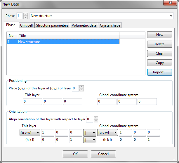
To create a new structure, choose the “File” menu \(\Rightarrow \) “New Structure…”. To edit current data, choose “Edit” menu \(\Rightarrow \) “Edit Data” \(\Rightarrow \) “Phase…”. In both of the cases, the same dialog box named New Data or Edit Data appears (Fig. 6.1). This dialog box consists of the following five tab pages:
- Phase
- Unit cell
- Structure parameters
- Volumetric data
- Crystal shape
At the top of the dialog box, a serial number and a title are displayed for the selected phase.
6.1 Defining Phases
In the Phase tab (Fig. 6.1) of the Edit Data dialog box, you can add, delete, copy, or import phase data that are overlaid on the same Graphics Area. To edit the title of a phase, select a row in the list and click on the Title column. When dealing with a single phase, you have nothing to do with this tab except for editing the title. The Positioning and Orientation frame boxes are used when superimposing two or more phases. See chapter 7 for how to visualize multiple phase data in the same Graphics Area.
6.2 Symmetry and Unit Cell
The Unit cell tab in the Edit Data dialog box is used to give lattice parameters and the symmetry of a structure (Fig. 6.2).
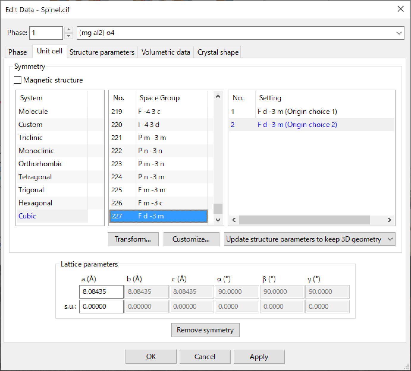
6.2.1 Crystal systems and space groups
Selection of crystal systems
The System list box is used to filter a list of space-group symbols in the Space group list box. When an item in this list box is selected, only space groups belonging to the selected crystal system will be highlighted in the Space group list box. The following ten items are listed in the System list box.
- Molecule
- Custom
- Triclinic
- Monoclinic
- Orthorhombic
- Tetragonal
- Trigonal
- Hexagonal
- Cubic
- Rhombohedral
On selection of Molecule, a Cartesian-coordinate system is used instead of fractional-coordinate system, which leads to the absence of “unit cell”. Therefore, text boxes and list boxes for settings of a space group and lattice parameters are disabled. When Custom is selected, space-group settings cannot be specified, but symmetry operations can be manually customized (see page 92).
Selection of a space group
Space group numbers and standard symbols are listed in the Space Group list box. Only space groups of a selected crystal system is highlighted in the list but you can select any space group. On selection of a space group, the list boxes of System and Setting will be updated.
Settings for a space group
The number of available settings for the selected space group is listed in list box Setting. Settings available in the list box are basically those compiled in International Tables for Crystallography, volume A [30].
In some space groups, additional settings are contained in list box {Setting}. In the triclinic system, complex lattices, \(A\), \(B\), \(C\), \(I\), \(F\), and \(R\), may be selected with setting numbers of 2, 3, 4, 5, 6, and 7, respectively (Table 6.1). In the monoclinic system, settings with unique axes \(a\), \(b\), and \(c\) are all available as built-in settings (Table 6.2).
In the orthorhombic system, any of six settings, i.e., \(\mathbf {abc}\), \(\mathbf {ba\overline {c}}\), \(\mathbf {cab}\), \(\mathbf {\overline {c}ba}\), \(\mathbf {bca}\), and \(\mathbf {a\overline {c}b}\) listed in Table 4.3.2.1 in Ref. [30] may be selected with setting numbers of 1, 2, 3, 4, 5, and 6, respectively. In orthorhombic space groups having two origin choices, odd and even setting numbers adopts origin choices 1 and 2, respectively. Then, settings 1 and 2 are of axis choice \(\mathbf {abc}\), settings 3 and 4 are of \(\mathbf {ba\overline {c}}\), and so on (Table 6.3).
On changes in crystal axes, e.g., rhombohedral or hexagonal axes in a trigonal crystal, lattice parameters are automatically converted.
When changing a setting number, consider whether you need to keep structure parameters or 3D geometries (see the following subsection).
| Setting number | Space group (\(P1\)) | Space group (\(P\overline {1}\)) |
|
|
|
|
| 1 | \(P1\) | \(P\overline {1}\) |
| 2 | \(A1\) | \(A\overline {1}\) |
| 3 | \(B1\) | \(B\overline {1}\) |
| 4 | \(C1\) | \(C\overline {1}\) |
| 5 | \(I1\) | \(I\overline {1}\) |
| 6 | \(F1\) | \(F\overline {1}\) |
| 7 | \(R1\) | \(R\overline {1}\) |
| Axis choice |
\(\mathbf {a\underline {b}c}\)
|
\(\mathbf {c\underline {\overline {b}}a}\)
|
\(\mathbf {ab\underline {c}}\)
|
\(\mathbf {ba\underline {\overline {c}}}\)
|
\(\mathbf {\underline {a}bc}\)
|
\(\mathbf {\underline {\overline {a}}cb}\)
|
||||||||||||
| Cell choice | 1 | 2 | 3 | 1 | 2 | 3 | 1 | 2 | 3 | 1 | 2 | 3 | 1 | 2 | 3 | 1 | 2 | 3 |
|
Unique axis \(b\)
|
Unique axis \(c\)
|
Unique axis \(a\)
|
||||||||||||||||
| \(P2\) | 1 | 2 | 3 | |||||||||||||||
| \(P2_1\) | 1 | 2 | 3 | |||||||||||||||
| \(C2\) | 1 | 2 | 3 | 4 | 5 | 6 | 7 | 8 | 9 | |||||||||
| \(Pm\) | 1 | 2 | 3 | |||||||||||||||
| \(Pc\) | 1 | 2 | 3 | 4 | 5 | 6 | 7 | 8 | 9 | |||||||||
| \(Cm\) | 1 | 2 | 3 | 4 | 5 | 6 | 7 | 8 | 9 | |||||||||
| \(Cc\) | 1 | 2 | 3 | 10 | 11 | 12 | 4 | 5 | 6 | 13 | 14 | 15 | 7 | 8 | 9 | 16 | 17 | 18 |
| \(P2/m\) | 1 | 2 | 3 | |||||||||||||||
| \(P2_1/m\) | 1 | 2 | 3 | |||||||||||||||
| \(C2/m\) | 1 | 2 | 3 | 4 | 5 | 6 | 7 | 8 | 9 | |||||||||
| \(P2/c\) | 1 | 2 | 3 | 4 | 5 | 6 | 7 | 8 | 9 | |||||||||
| \(P2_1/c\) | 1 | 2 | 3 | 4 | 5 | 6 | 7 | 8 | 9 | |||||||||
| \(C2/c\) | 1 | 2 | 3 | 10 | 11 | 12 | 4 | 5 | 6 | 13 | 14 | 15 | 7 | 8 | 9 | 16 | 17 | 18 |
|
Space groups
|
|||
| Axis choice |
No. 48, 50, 59, 68, and 70
|
Others | |
| Origin choice 1 | Origin choice 2 | ||
| \(\mathbf {abc}\) | 1 | 2 | 1 |
| \(\mathbf {ba\overline {c}}\) | 3 | 4 | 2 |
| \(\mathbf {cab}\) | 5 | 6 | 3 |
| \(\mathbf {\overline {c}ba}\) | 7 | 8 | 4 |
| \(\mathbf {bca}\) | 9 | 10 | 5 |
| \(\mathbf {a\overline {c}b}\) | 11 | 12 | 6 |
6.2.2 Behavior when changing a space-group setting
The list box below the Setting controls the behavior when changing a space-group setting. There are two options:
- Update structure parameters to keep 3D geometry
- Keep structure parameters unchanged
On the use of the first option (default), lattice parameters and fractional coordinates are converted to keep the structural geometry of a crystal when the setting number of a space group is changed or a transformation matrix is specified. When the second option is used, lattice parameters and fractional coordinates remain unchanged instead of the geometry.
If a correct structure is displayed in the Graphic Area but another space-group setting is preferred to the current one, choose Update structure parameters to keep 3D geometry and change the space-group setting. The second option is typically used to change a setting number when the correct setting number is not recognized by VESTA after reading in a file such as CIF. In such a case, lattice parameters and fractional coordinates are correct whereas symmetry operations are incorrect. Then, choose Keep structure parameters unchanged and select the correct setting number. When a setting number cannot be uniquely determined from data recorded in a structural-data file, VESTA assumes setting number 2 (a setting with the inversion center at the origin) in centrosymmetric space groups with two origin choices, and setting number 1 in all the other space groups.
Note that even if structure parameters remain unchanged, some lattice parameters may be changed in conformity with constraints imposed on them in the current space-group setting.
6.2.3 Lattice parameters
In the Lattice parameters frame box, lattice parameters are input in the unit of Å (\(a\), \(b\), and \(c\)) and degrees (\(\alpha \), \(\beta \), and \(\gamma \)). Lattice parameters input by the user are automatically constrained on the basis of a crystal system. Standard uncertainties (s.u.’s) of lattice parameters are used to calculate s.u.’s of geometrical parameters. For structural data based on the Cartesian coordinates (when Molecule is selected as the Crystal system), text boxes in this frame box are disabled.
6.2.4 Customization of symmetry operations
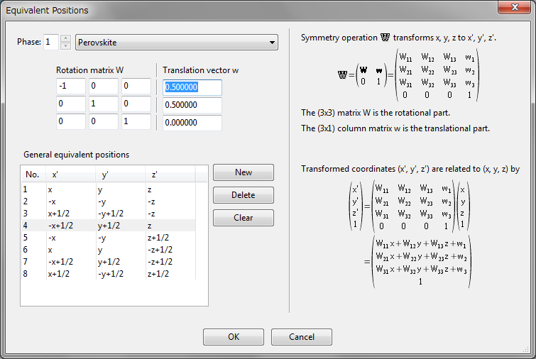
To customize symmetry operations, click the [Customize…] button. Then, the Equivalent Positions dialog box appears with an editing mode (Fig. 6.3), and a list of general equivalent positions is displayed in this dialog box. When one of the equivalent positions in the list is selected, the corresponding symmetry operation is displayed in a matrix form at the upper left of the dialog box. If you input a value in one of the text boxes, representation of the corresponding equivalent position in the list is updated. To add a new symmetry operation, click the [New] button. To remove a symmetry operation, select an item in the list and click the [Delete] button. Clicking the [Clear] button removes all the symmetry operations other than the identity operation.
6.2.5 Reducing symmetry
Clicking the [Remove symmetry] button generates all the atoms in the unit cell as virtual independent sites by reducing the symmetry of the crystal to \(P1\). When the space group is changed to that with higher symmetry, or when the unit cell is transformed to a smaller one (see 6.2.6), the same atomic position may result from two or more sites. In such a case, the redundant sites can be removed by clicking the [Remove duplicate atoms] button in the Structure parameters tab (see page 124).
6.2.6 Transformation of the unit cell
Clicking the [Transform...] button opens the Unit Cell Transformation dialog box (Fig. 6.4). This dialog box allow you to transform crystal axes by specifying \(3 \times 3\) rotation matrix \(\bm {P}\) and \(3 \times 1\) translation vector \(\bm {p}\). The [View general positions] button in the dialog box is used to open the Equivalent Positions dialog box to check the general equivalent positions and symmetry operations of the transformed unit cell (see 14.1). Clicking the [Initialize current matrix] button resets the transformation matrix to the identity matrix. Currently, this operation cannot be canceled. When option “Normalize the fractional coordinates” is checked, new atomic coordinates of the transformed unit cell will be normalized within a range of 0 to 1.
In what follows, a more detailed explanation and use cases of the Unit Cell Transformation dialog box will be given.
![]()
Non-conventional space-group settings
To convert a structure from a conventional setting to a non-conventional one, you have to select a mode Update structure parameters to keep 3D geometry in the Unit cell tab of the Edit Data dialog box before opening the Unit Cell Transformation dialog box. With this mode, both lattice parameters and fractional coordinates are automatically transformed into new ones to keep the current geometry of the crystal structure. When the mode Keep structure parameters unchanged is selected, only symmetry operations are transformed to those of the new setting, whereas lattice parameters and fractional coordinates remain unchanged.
The new origin of the transformed unit cell is specified as the origin shift \(\bm {p}\). For instance, if you specify \((0.25, 0.25, 0.25)\) as an origin shift, a coordinate of \((0.25, 0.25, 0.25)\) of a conventional setting becomes \((0, 0, 0)\) of the transformed non-conventional unit-cell.
Orientations of the transformed crystal axes \(\bm {a}'\), \(\bm {b}'\), and \(\bm {c}'\) are specified as column vectors in the \(3 \times 3\) rotation matrix \(\bm {P}\), i.e., the first, second, and third columns of \(\bm {P}\) represent \(\bm {a}'\), \(\bm {b}'\), and \(\bm {c}'\) respectively. For example, the following transformation matrix is used to swap the \(a\) and \(b\) axes. \begin {equation} \begin {split} \bm {P} &= \begin {pmatrix} 0 & 1 & 0\\ 1 & 0 & 0\\ 0 & 0 & -1\end {pmatrix} . \end {split} \end {equation} Note that the orientation of the \(c\) axis is inverted in this case, or otherwise the transformed structure becomes enantiomorphic with respect to the original structure in non-centrosymmetric space groups. In general, when the determinant of \(\bm {P}\), det(\(\bm {P}\)), is negative, the crystal-coordinate system is transformed from right-handed to left-handed, and vice versa. When such a matrix is specified as \(\bm {P}\), a warning dialog box will appear to confirm whether or not you proceed to the next step.
![]()
The unit-cell volume, \(V\), is transformed to \(V'\) by \begin {equation} V' = \mathrm {det} ( \bm {P} ) V . \end {equation} Therefore, the unit-cell volume changes on the transformation unless det(\(\bm {P}\)) is 1.
The entire transformation including both a rotation and an origin shift can be expressed by single \(4 \times 4\) transformation matrix \(\mathbb {P}\), which consists of the \(3 \times 3\) rotation matrix \(\bm {P}\), the \(3 \times 1\) translation vector \(\bm {p}\), and the row vector \(\bm {o}\) = (0, 0, 0) [50]: \begin {equation} \begin {split} \mathbb {P} &= \begin {pmatrix} \bm {P} & \bm {p} \\ \bm {o} & 1\end {pmatrix} = \begin {pmatrix} P_{11} & P_{12} & P_{13} & p_1\\ P_{21} & P_{22} & P_{23} & p_2\\ P_{31} & P_{32} & P_{33} & p_3\\ 0 & 0 & 0 & 1\end {pmatrix} . \end {split} \end {equation} Then each of the following crystallographic variables, i.e., primitive translation vectors \(\bm {a}\), \(\bm {b}\), \(\bm {c}\), reciprocal lattice vectors \(\bm {a}^*\), \(\bm {b}^*\), \(\bm {c}^*\), metric tensor \(\bm {G}\), metric tensor of reciprocal lattice \(\bm {G}^*\), atomic coordinate \(\bm {X}\), symmetry operation \(\mathbb {W}\), and anisotropic atomic displacement parameters \(\bm {\beta }\), are transformed as described below.
Primitive translation vectors \(\bm {a}\), \(\bm {b}\) and \(\bm {c}\) are transformed by \(\bm {P}\) as \begin {equation} \begin {split} (\bm {a}', \bm {b}', \bm {c}') &= (\bm {a}, \bm {b}, \bm {c}) \bm {P} \\[5pt] &= (\bm {a}, \bm {b}, \bm {c}) \begin {pmatrix} P_{11} & P_{12} & P_{13} \\ P_{21} & P_{22} & P_{23} \\ P_{31} & P_{32} & P_{33} \end {pmatrix} \\[5pt] &= ( P_{11}\bm {a} + P_{21}\bm {b} + P_{31}\bm {c}, \, P_{12}\bm {a} + P_{22}\bm {b} + P_{32}\bm {c}, \, P_{13}\bm {a} + P_{23}\bm {b} + P_{33}\bm {c} ). \end {split} \label {eq:transformation-by-P} \end {equation}
The shift of the origin, i.e., (0, 0, 0), is defined with a shift vector \(\bm {t}\) as \begin {equation} \begin {split} \bm {t} &= (\bm {a}, \bm {b}, \bm {c}) \bm {p} \\[5pt] &= (\bm {a}, \bm {b}, \bm {c}) \begin {pmatrix} p_{1} \\ p_{2} \\ p_{3}\end {pmatrix} \\[5pt] &= p_1 \bm {a} + p_2 \bm {b} + p_3 \bm {c} . \end {split} \end {equation}
Let \(\bm {A}\) be the representation matrix of primitive translation vectors, \(\bm {a}\), \(\bm {b}\), and \(\bm {c}\), on the basis of a set of orthonormal vectors, \(\bm {x}\), \(\bm {y}\), and \(\bm {z}\): \begin {equation} \bm {A} = (\bm {a}, \bm {b}, \bm {c}) = \begin {pmatrix} a_{x} & b_{x} & c_{x}\\ a_{y} & b_{y} & c_{y}\\ a_{z} & b_{z} & c_{z}\end {pmatrix} . \end {equation} Then the transformation by Eq. \eqref{eq:transformation-by-P} can be rewritten as \begin {equation} \bm {A}' = \bm {A} \bm {P} . \end {equation}
Alternatively, the use of the metric tensor, \(\bm {G}\), is often preferable to the direct use of \(\bm {A}\) owing to the unique definition of \(\bm {G}\). On the other hand, the number of representations for \(\bm {A}\) is infinite because the orthonormal bases, \(\bm {x}\), \(\bm {y}\), and \(\bm {z}\), may be arbitrarily chosen. The metric tensor (matrix) of the direct lattice is defined as \begin {equation} \bm {G} = \bm {A}^\mathrm {t} \bm {A} = \begin {pmatrix} \bm {a}\cdot \bm {a} & \bm {a}\cdot \bm {b} & \bm {a}\cdot \bm {c} \\ \bm {b}\cdot \bm {a} & \bm {b}\cdot \bm {b} & \bm {b}\cdot \bm {c} \\ \bm {c}\cdot \bm {a} & \bm {c}\cdot \bm {b} & \bm {c}\cdot \bm {c} \\ \end {pmatrix} = \begin {pmatrix} a^2 & ab \cos \gamma & ac \cos \beta \\ ba \cos \gamma & b^2 & bc \cos \alpha \\ ca \cos \beta & cb \cos \alpha & c^2 \end {pmatrix} , \label {eq:G} \end {equation} where \(\mathrm {t}\) denotes transposition. Then, \(\bm {G}\) is transformed into \(\bm {G}'\) by \begin {equation} \bm {G}' = (\bm {A}')^\mathrm {t} \bm {A}' = (\bm {A P})^\mathrm {t} (\bm {A P}) = \bm {P}^\mathrm {t} (\bm {A}^\mathrm {t} \bm {A}) \bm {P} = \bm {P}^\mathrm {t} \bm {G} \bm {P} . \end {equation} Similarly, the representation matrix of the reciprocal basis vectors \(\bm {a}^*\), \(\bm {b}^*\), and \(\bm {c}^*\) is defined as \begin {equation} \bm {A}^* = (\bm {a}^*, \bm {b}^*, \bm {c}^*) = \begin {pmatrix} a^*_{x} & b^*_{x} & c^*_{x}\\ a^*_{y} & b^*_{y} & c^*_{y}\\ a^*_{z} & b^*_{z} & c^*_{z}\end {pmatrix} . \end {equation} The direct and reciprocal basis vectors are related by \begin {equation} \bm {A}^* = (\bm {A}^{-1})^\mathrm {t} = (\bm {A}^\mathrm {t})^{-1} \end {equation} and \begin {equation} (\bm {A}^*)^\mathrm {t} \bm {A} = \bm {A} (\bm {A}^*)^\mathrm {t} = \bm {A}^* \bm {A}^\mathrm {t} = \bm {A}^\mathrm {t} \bm {A}^* = \bm {E} , \end {equation} where \(\bm {E}\) is the identity matrix: \begin {equation} \bm {E} = \begin {pmatrix} 1 & 0 & 0\\ 0 & 1 & 0\\ 0 & 0 & 1\end {pmatrix} . \end {equation} The metric tensor of the reciprocal lattice is defined as \begin {equation} \bm {G}^* = (\bm {A}^*)^\mathrm {t} \bm {A}^* = \begin {pmatrix} \bm {a}^*\cdot \bm {a}^* & \bm {a}^*\cdot \bm {b}^* & \bm {a}^*\cdot \bm {c}^* \\ \bm {b}^*\cdot \bm {a}^* & \bm {b}^*\cdot \bm {b}^* & \bm {b}^*\cdot \bm {c}^* \\ \bm {c}^*\cdot \bm {a}^* & \bm {c}^*\cdot \bm {b}^* & \bm {c}^*\cdot \bm {c}^* \\ \end {pmatrix} = \begin {pmatrix} a^{*2} & a^* b^* \cos \gamma ^* & a^* c^* \cos \beta ^* \\ b^* a^* \cos \gamma ^* & b^{*2} & b^* c^* \cos \alpha ^* \\ c^* a^* \cos \beta ^* & c^* b^* \cos \alpha ^* & c^{*2} \end {pmatrix} . \label {eq:G_star} \end {equation} The transformation of \(\bm {G}^*\) into \({\bm {G}^*}'\) is represented by \begin {equation} {\bm {G}^*}' = ({\bm {A}^*}')^\mathrm {t} {\bm {A}^*}' = (\bm {A P})^{-1} ((\bm {A P})^\mathrm {t})^{-1} = \bm {P}^{-1} ((\bm {A}^*)^\mathrm {t} \bm {A}^*) (\bm {P}^{-1})^\mathrm {t} = \bm {Q} \bm {G}^* \bm {Q}^\mathrm {t} , \end {equation} where \(\bm {Q} = \bm {P}^{-1}\).
The coordinates \(x\), \(y\), and \(z\) in the direct space are transformed by the \(4 \times 4\) transformation matrix \(\mathbb {Q}\) as \begin {equation} \begin {pmatrix} x' \\ y' \\ z' \\ 1\end {pmatrix} = \mathbb {Q} \begin {pmatrix} x \\ y \\ z \\ 1\end {pmatrix}, \label {eq:qx} \end {equation} where \begin {equation} \begin {split} \mathbb {Q} &= \begin {pmatrix} \bm {P}^{-1} & -\bm {P}^{-1} \bm {p} \\ \bm {o} & 1\end {pmatrix} \\[5pt] & = \begin {pmatrix} \bm {Q} & \bm {q} \\ \bm {o} & 1\end {pmatrix} \\[5pt] & = \begin {pmatrix} Q_{11} & Q_{12} & Q_{13} & q_1\\ Q_{21} & Q_{22} & Q_{23} & q_2\\ Q_{31} & Q_{32} & Q_{33} & q_3\\ 0 & 0 & 0 & 1\end {pmatrix}\\[5pt] &= \mathbb {P}^{-1} . \end {split} \label {eq:Q-matrix} \end {equation} In short, Eq. \eqref{eq:qx} can be expressed as: \begin {equation} \bm {X}' = \mathbb {Q}\bm {X}. \end {equation} The \(4 \times 4\) symmetry operation matrix \(\mathbb {W}\) transforms the coordinates \(x\), \(y\), and \(z\), of point \(\bm {X}\) to a symmetrically equivalent point \(\bm {\widetilde {X}}\) with the coordinates, \(\tilde {x}\), \(\tilde {y}\), and \(\tilde {z}\), by \begin {equation} \begin {split} \begin {pmatrix} \tilde {x} \\ \tilde {y} \\ \tilde {z} \\ 1\end {pmatrix} &= \begin {pmatrix} W_{11} & W_{12} & W_{13} & w_1\\ W_{21} & W_{22} & W_{23} & w_2\\ W_{31} & W_{32} & W_{33} & w_3\\ 0 & 0 & 0 & 1\end {pmatrix} \begin {pmatrix} x \\ y \\ z \\ 1\end {pmatrix} \\[5pt] &= \begin {pmatrix} W_{11} x + W_{12} y + W_{13} z + w_1\\ W_{21} x + W_{22} y + W_{23} z + w_2\\ W_{31} x + W_{32} y + W_{33} z + w_3\\ 1\end {pmatrix} , \label {eq:wx} \end {split} \end {equation} or in short notation, \begin {equation} \bm {\widetilde {X}} = \mathbb {W}\bm {X}. \end {equation} The matrix \(\mathbb {Q}\) transforms both \(\bm {X}\) and \(\bm {\widetilde {X}}\) to \(\bm {X}'\) and \(\bm {\widetilde {X}}'\), respectively:
Let \(\bm {Q}^{\mathrm {t}}\) be the transposed matrix of \(\bm {Q}\) defined in Eq. \eqref{eq:Q-matrix}. Then, anisotropic atomic displacement parameters, \(\bm {\beta }\), are transformed by \begin {equation} \begin {split} \bm {\beta }' &= \begin {pmatrix} \beta _{11}' & \beta _{12}' & \beta _{13}' \\ \beta _{12}' & \beta _{22}' & \beta _{23}' \\ \beta _{13}' & \beta _{23}' & \beta _{33}' \end {pmatrix}\\[5pt] &= \begin {pmatrix} Q_{11} & Q_{12} & Q_{13} \\ Q_{21} & Q_{22} & Q_{23} \\ Q_{31} & Q_{32} & Q_{33} \end {pmatrix} \begin {pmatrix} \beta _{11} & \beta _{12} & \beta _{13} \\ \beta _{12} & \beta _{22} & \beta _{23} \\ \beta _{13} & \beta _{23} & \beta _{33} \end {pmatrix} \begin {pmatrix} Q_{11} & Q_{21} & Q_{31} \\ Q_{12} & Q_{22} & Q_{32} \\ Q_{13} & Q_{23} & Q_{33} \end {pmatrix}\\[5pt] &= \bm {Q \beta Q}^\mathrm {t} . \end {split} \end {equation}
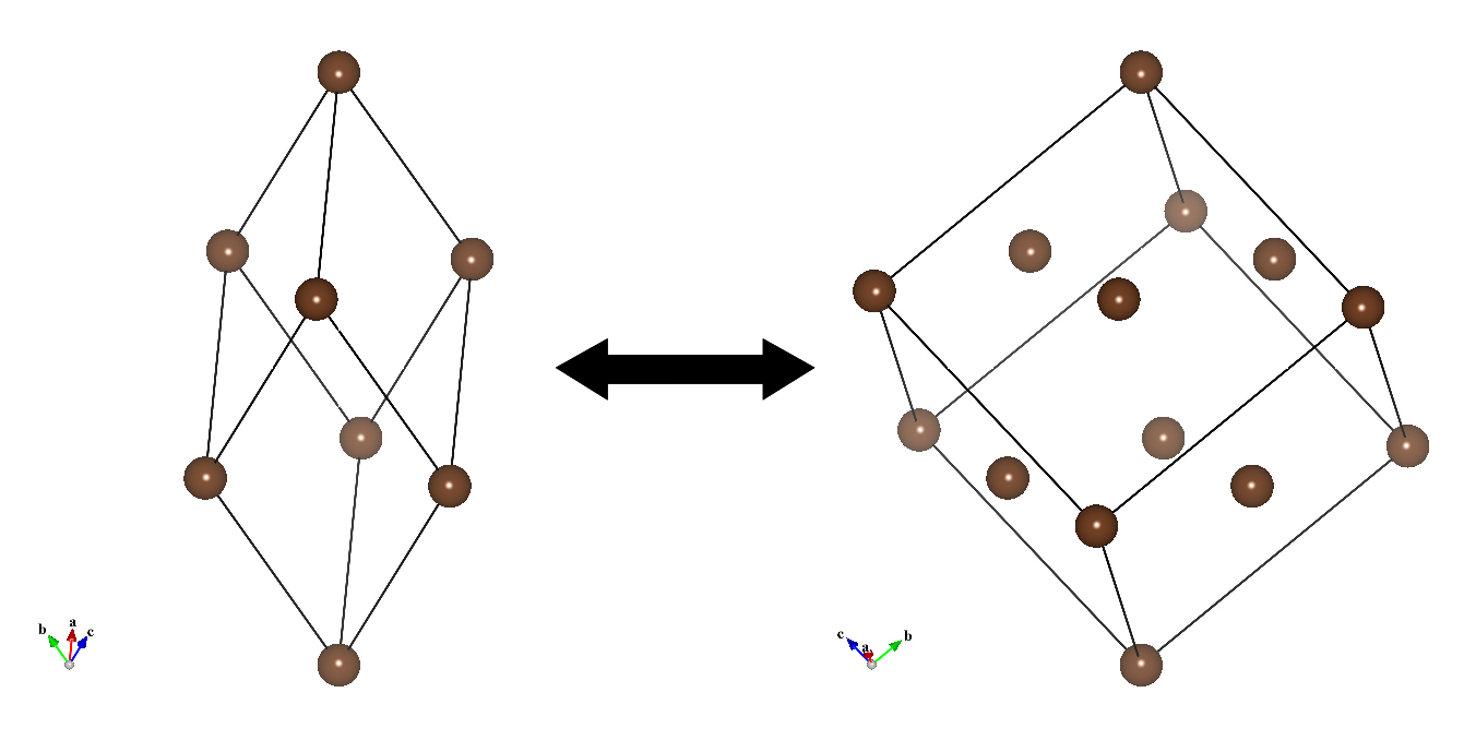
Creation of superstructures and substructures
The transformation matrix is also used to convert (primitive lattice)\(\rightleftarrows \)(complex lattice) (Fig. 6.6), and to create superstructures and averaged substructures. To convert a structure, you have to select mode Update structure parameters to keep 3D geometry in the Unit cell tab of the Edit Data dialog box before opening the Unit Cell Transformation dialog box.
When the determinant of \(\bm {P}\), det(\(\bm {P}\)) is larger than 1, the transformed unit-cell becomes larger than the original one, and when det(\(\bm {P}\)) is smaller than 1, the transformed unit-dell becomes smaller than the original one. In such cases, a dialog box appears to confirm whether you intend to change the unit cell volume (Fig. 6.7).
![]()
When a rotation matrix with det(\(\bm {P}\)) \(> 1\) is specified, or the transformed unit cell contains additional lattice points even when det(\(\bm {P}\)) \(= 1\), a dialog box appears to ask you how to convert the structure (Fig. 6.8). There are the following three options:
- “Add new equivalent positions to a list of symmetry operations”
- “Search atoms in the new unit cell and add them as new sites”
- “Do nothing”
![]()
In the first and second options, the structural geometry of the original data will remain unchanged. On the other hand, on selection of the third option, some atoms in the new unit cell will be missing. On selection of the first option, a superstructure will be created by examining the following equation to find additional symmetry operations \(\mathbb {W}'\) having a translational component in between (0, 0, 0) and (1, 1, 1): \begin {equation} \begin {split} \mathbb {W}' = \begin {pmatrix} W'_{11} & W'_{12} & W'_{13} & w'_1\\ W'_{21} & W'_{22} & W'_{23} & w'_2\\ W'_{31} & W'_{32} & W'_{33} & w'_3\\ 0 & 0 & 0 & 1\end {pmatrix} = \mathbb {Q} \begin {pmatrix} W_{11} & W_{12} & W_{13} & w_1 + n_x\\ W_{21} & W_{22} & W_{23} & w_2 + n_y\\ W_{31} & W_{32} & W_{33} & w_3 + n_z\\ 0 & 0 & 0 & 1\end {pmatrix} \mathbb {P},\\ \mspace {60mu}(n_x, n_y, n_z = 0, \pm 1, \pm 2, \dots ). \end {split} \end {equation}
On selection of the second option, a superstructure will be created by examining the following equation to find additional sites lying in between (0, 0, 0) and (1, 1, 1): \begin {equation} \begin {pmatrix} x' \\ y' \\ z' \\ 1\end {pmatrix} = \mathbb {Q} \begin {pmatrix} x+n_x\\ y+n_y \\ z+n_z \\ 1\end {pmatrix}. \mspace {60mu}(n_x, n_y, n_z = 0, \pm 1, \pm 2, \dots ) \end {equation}
Note that the transformed new unit-cell should be symmetrically consistent with the space group currently in use. Otherwise, reduce symmetry to \(P1\) by clicking [Remove symmetry] before creating a superstructure, and input a new space group after the superstructure has been created. If det(\(\bm {P}\)) \(<\) 1, the same position may result from two or more sites. In such a case, the redundant sites can be removed by clicking [Remove duplicate atoms] button in the Structure parameters tab (see page 124).
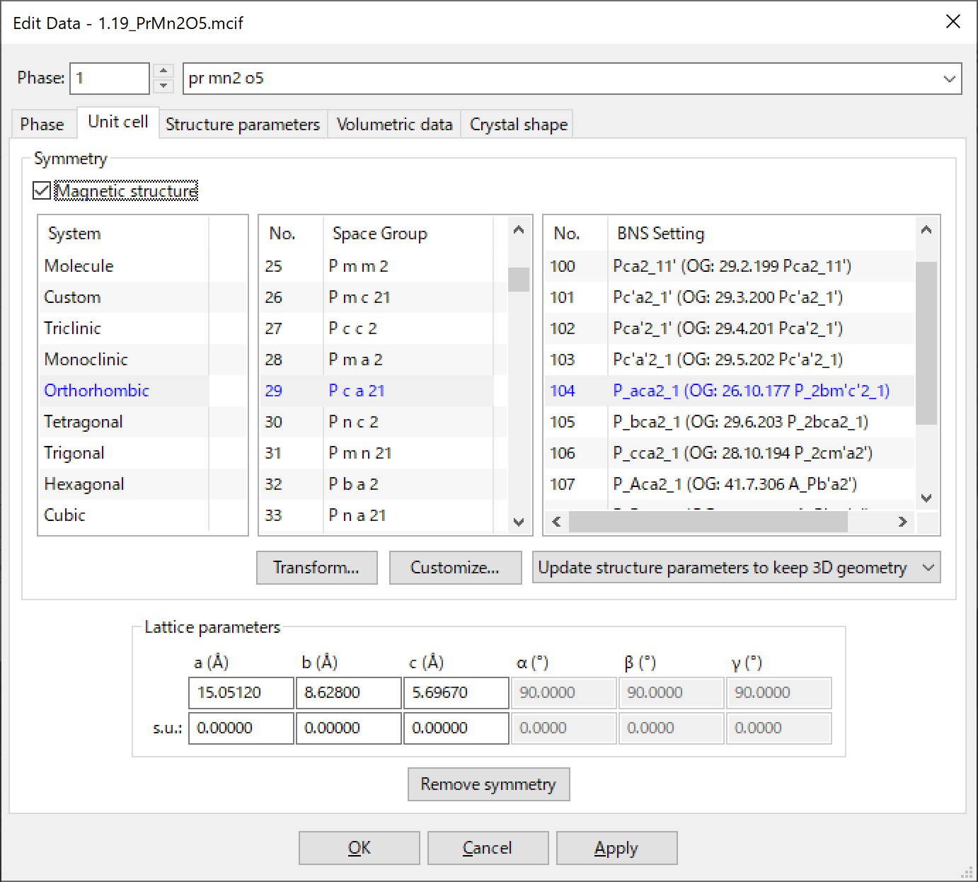
6.2.7 Magnetic Structures
VESTA fully supports 1651 magnetic space groups. Check the “Magnetic structure” check box to use magnetic space groups. Then, the title of the Setting list box changes to BNS Setting, which shows a list of magnetic space groups for a selected space group. There are two types of notations of magnetic space groups: the Belov–Neronova–Smirnova (BNS) notation [51] and the Opechowski–Guccione (OG) notation [52]. VESTA uses the BNS notation because symmetry operations of the BNS notation are described with respect to the magnetic unit-cell with translational parts never exceeding 1. Atomic coordinates, displacement parameters, and occupancies of a magnetic structure are specified exactly the same way as conventional structure (see Section 6.3). Magnetic moments of atoms are specified in the Vectors dialog box (see Section 9.1).
6.3 Structure Parameters
The Structure parameters tab in the Edit Data dialog box (Fig. 6.10) is used to input and edit parameters related to atomistic structures. The following structural information is input or edited by using text boxes at the upper half of the page:
- [Symbol...]: Symbol of an element (up to two characters).
- {Label}: Site name (up to six characters).
- {Charge}: Formal charge (oxidation number; optional)
- {x}, {y}, and {z}: Fractional coordinates, \(x\), \(y\), and \(z\) (dimensionless).
- {s.u.(x)}, {s.u.(y)}, and {s.u.(z)}: Standard uncertainties of the fractional coordinates (default values: zero).
- {Occ}: Occupancy (dimensionless; optional).
- {B} or {U}: Isotropic atomic displacement parameter, \(B\) or \(U\) (in Å\(^2\); optional).
- {U11}, {U22}, {U33}, {U12}, {U13}, and {U23}: Anisotropic atomic displacement parameters, \(U_{ij}\) (in Å\(^2\), optional).
- {beta11}, {beta22}, {beta33}, {beta12}, {beta13}, and {beta23}: Anisotropic atomic displacement parameters, \(\beta _{ij}\) (dimensionless; optional).
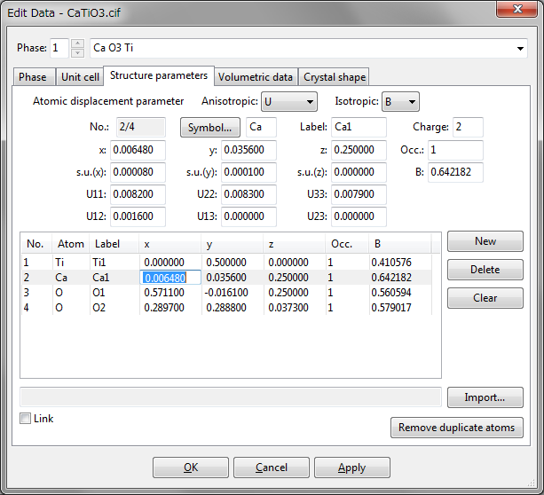
A list of sites in the asymmetric unit is shown at the lower half of the page. Text boxes are disabled when no site is selected in the list. When an item in the list is selected, the text boxes are updated to show data relevant to the selected site. In-place editing of a list item is also supported, as Fig. 6.10 shows.
To add a new site, click the [New] button at first, and edit texts in the text boxes. A modification in a text box is applied to the selected site immediately after the focus (caret) has moved to another text box or another GUI control. In the case of text boxes for numerical values, modifications will be discarded if an input text is not a valid numerical value, or if the text box is empty. Therefore, if you have accidentally changed a value in a text box, the original value can be restored by erasing the entire text in the text box before moving the focus to another GUI control.
To delete a site, select an item in the list, and click the [Delete] button or press the \(<\)Delete\(>\) key. Clicking the [Clear] button will delete all the sites in the list.
6.3.1 Symbols and Labels
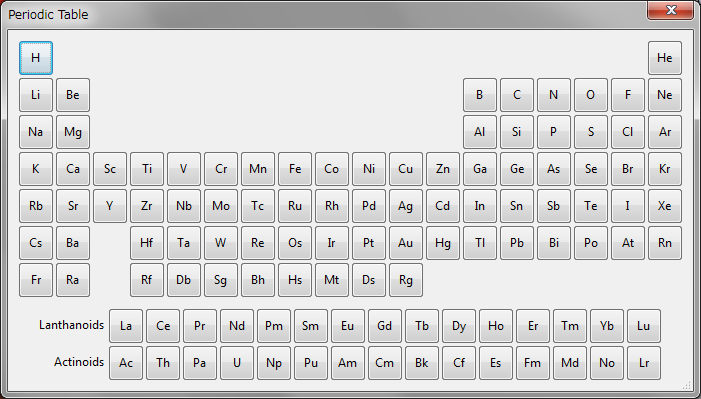
Up to two characters are input as an element symbol while up to nine characters are input as a label of a site. Click the [Symbol…] button to select an element symbol from the Periodic Table dialog box (Fig. 6.11).
6.3.2 Formal charge
Strictly speaking, formal charges are not structure parameters. They are, however, used to estimate a bond length from a bond valence parameter [38, 39, 40] (see 11.4.3), evaluate charge distribution from bond lengths [35, 36, 37] (see 11.4.3), and calculate electrostatic site potentials and a Madelung energy by the Fourier method (see 14.5).
6.3.3 Fractional coordinates
For special positions, input fractional numbers, e.g., 1/4, 1/2, and 1/3, or a sufficient number of digits should be given, e.g., 0.333333 and 0.666667.
When displacement ellipsoids are drawn from anisotropic atomic displacement parameters refined with RIETAN-FP [12], fractional coordinates corresponding to the first equivalent position described in International Tables for Crystallography, volume A [30] for each Wyckoff position have to be entered. For example, input not (1/2, 0, \(z\)) but (0, 1/2, \(z\)) for a 4\(i\) site in space group \(P\)4/\(mmm\) (No. 123).
6.3.4 Occupancy
The occupancy is unity for full occupation and zero for virtual sites. If the occupancy of a site is less than unity, atoms occupying there are displayed as circle graphs for occupancies. If unicolor balls are preferred to bicolor ones, change the occupancy to unity for convenience.
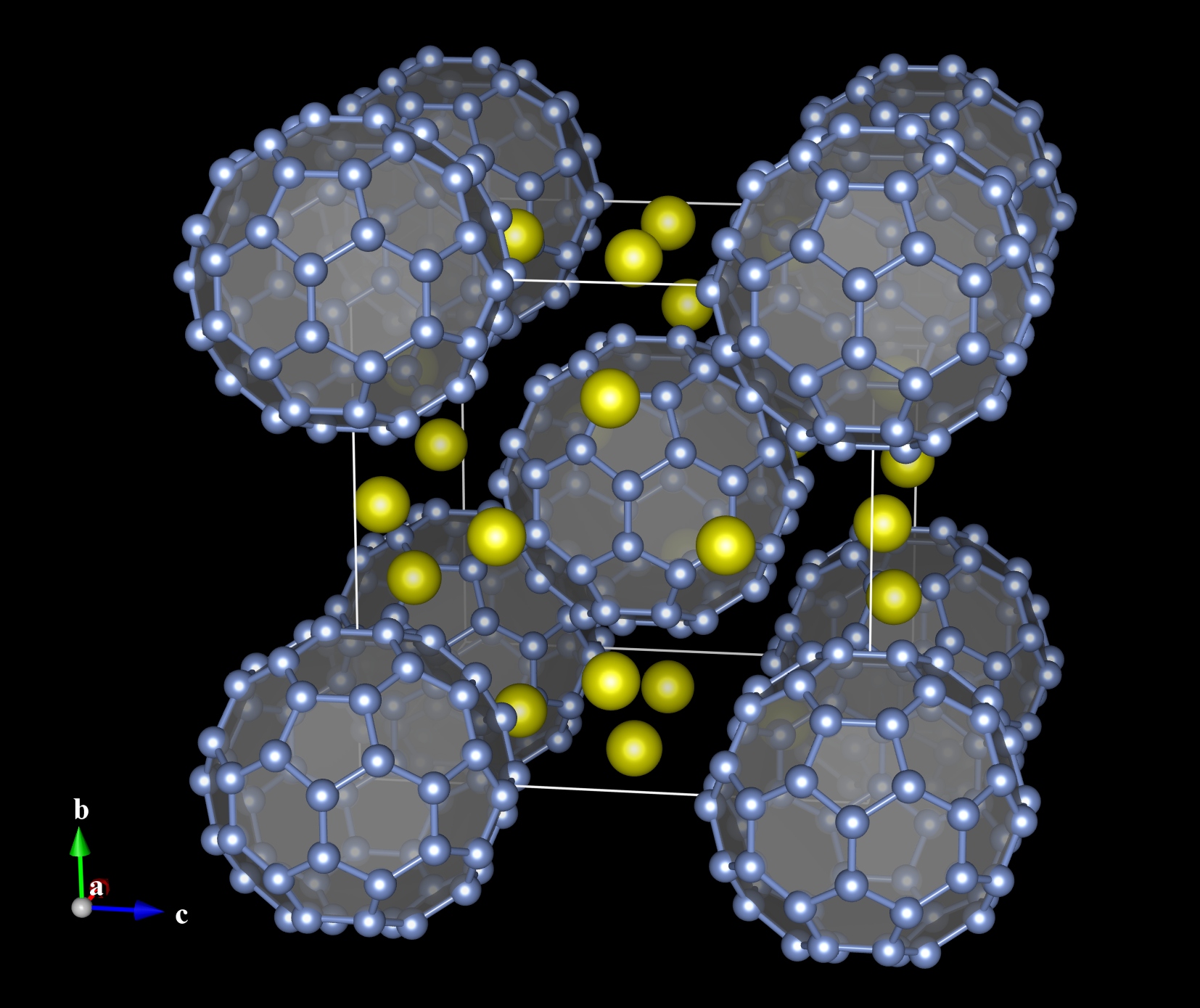
If the occupancy of a site is zero, the site is treated as a virtual site that is not occupied by any atoms in the real structure. Neither the virtual sites nor bonds connecting them are displayed on the screen. Virtual sites are used to visualize, for example, cage structures of porous crystals as solid polyhedra without creating a large number of unnecessary bonds (Fig. 6.12).
6.3.5 Atomic displacement parameters
The Debye–Waller factor, \(T_j (\bm {h})\), which is often referred to as the temperature factor, is included in formulae for structure factors, \(F(\bm {h})\), to represent the effect of static and dynamic displacement of atom \(j\) (see section 14.7). The displacement of atom is formulated in two different ways: anisotropic and isotropic atomic displacement.
Anisotropic models
The anisotropic Debye–Waller factor, \(T(\bm {h})\), is defined as \begin {equation} \begin {split} T(\bm {h}) &= \exp \left [ -2\pi ^2 \left ( h^2 a^{*2} U_{11} + k^2 b^{*2} U_{22} + l^2c^{*2} U_{33} + 2hk a^*b^*U_{12} + 2hl a^*c^*U_{13} + 2kl b^*c^*U_{23} \right ) \right ] \\[3pt] &= \exp \left [-\left ( h^2 \beta _{11} + k^2 \beta _{22} + l^2 \beta _{33} + 2hk\beta _{12} + 2hl\beta _{13} + 2kl\beta _{23}\right ) \right ] , \end {split} \end {equation} where \(a^*, b^*, c^*, \alpha ^*, \beta ^*\), and \(\gamma ^*\) are reciprocal lattice parameters.
The type of anisotropic atomic displacement parameters must be specified in list box {Anisotropic}: ‘None’ to omit anisotropic atomic displacement parameters, ‘U’ to input \(U_{ij}\) (\(U_{11}\), \(U_{22}\), \(U_{33}\), \(U_{12}\), \(U_{13}\), and \(U_{23}\)), and ‘beta’ to input \(\beta _{ij}\) (\(\beta _{11}\), \(\beta _{22}\), \(\beta _{33}\), \(\beta _{12}\), \(\beta _{13}\), and \(\beta _{23}\)). Using this list box, we can convert \(U_{ij}\) into \(\beta _{ij}\) and vice versa.
Anisotropic atomic displacement parameters defined in different ways must be converted into \(U_{ij}\) or \(\beta _{ij}\) defined above.
On refinement of \(\beta _{ij}\)’s by the Rietveld method with RIETAN-FP [12], \(\beta _{ij}\)’s for each site have to satisfy linear constraints imposed on them [54, 55].
Isotropic models
The isotropic Debye–Waller factor, \(T(\bm {h})\), is given by \begin {equation} \begin {split} T(\bm {h}) &= \exp \left [-B\left (\frac {\sin \theta }{\lambda }\right )^2\right ]\\[3pt] &= \exp \left (-\frac {B}{4d^2}\right )\\[3pt] &= \exp \left (-\frac {2\pi ^2U}{d^2}\right ), \end {split} \end {equation} where \(B\) and \(U\) are the isotropic atomic displacement parameters (\(U = B/8\pi ^2\)), \(\theta \) is the Bragg angle, \(\lambda \) is the X-ray or neutron wavelength, and \(d\) is the lattice-plane spacing. \(B\) and \(U\) are related to the mean square displacement, \(\bigl \langle u^2 \bigr \rangle \), along the direction perpendicular to the reflection plane with \begin {equation} B = 8\pi ^2 U = 8\pi ^2 \bigl \langle u^2 \bigr \rangle . \end {equation} For example, a \(B\) value of 3 Å\(^2\) corresponds to a displacement of about 0.2 Å.
The type of isotropic atomic displacement parameters must be specified in list box {Isotropic}. Using this list box, we can convert \(U\) into \(B\) and vice versa.
Isotropic atomic displacement parameters defined in different ways must be converted into \(B\) or \(U\) defined above.
In crystallographic sites for which anisotropic atomic displacement parameters, \(U_{ij}\) or \(\beta _{ij}\), have been input, equivalent isotropic atomic displacement parameters, \(B_{\mathrm {eq}}\) or \(U_{\mathrm {eq}}\), are calculated from \(U_{ij}\), \(a^*\), \(b^*\), \(c^*\), and the metric tensor \(\bm {G}\) [56, 57]: \begin {equation} B_\mathrm {eq} = 8\pi ^2 U_\mathrm {eq} \end {equation} with \begin {equation} \begin {split} U_\mathrm {eq} &= \frac {1}{3} \textstyle \sum _i \sum _j U_{ij} a_i^* a_j^* \bm {a}_i \cdot \bm {a}_j \\ &= \frac {1}{3} \bigl [ U_{11} \left ( a a^* \right )^2 + U_{22} \left ( b b^* \right )^2 + U_{33} \left ( c c^* \right )^2 \bigr . \\ &\quad + \bigl . 2U_{12} a^* b^* ab \cos \gamma + 2U_{13} a^* c^* ac \cos \beta + 2U_{23} b^* c^* bc \cos \alpha \bigr ] . \end {split} \end {equation} \(B_{\mathrm {eq}}\) and \(U_{\mathrm {eq}}\) are regarded as \(B\) and \(U\) in the Structure parameters tab of the Edit Data dialog box after reopening it.
6.3.6 Importing structure parameters
Structure parameters can be imported from a file storing structure parameters by clicking the [Import…] button at the bottom right of the Structure parameters page. Then, select a file with a format supported by VESTA in the file selection dialog box.
Option “Link” specifies the manner of outputting current structure data in a file, *.vesta, with the VESTA format. Structure data are usually recorded in *.vesta. On the other hand, for volumetric data, relative paths (including a file name) of data files are recorded in *.vesta instead of recording the volumetric data directly in it. When option “Link” is checked, structural data are also recorded as the relative path of the data file. Then, even if the structural-data file is changed after saving *.vesta, the changes are reflected in VESTA when *.vesta is reopened. This option is useful in preparing a file, *.vesta, with the VESTA format as a template file for setting objects and overall appearances. This option disables text boxes and list boxes in the Structure parameters tab to prohibit users from editing structure data because any modifications to structure data will not be saved to a file when this option is enableld.
6.3.7 Removing duplicate atoms
When the space group is changed to that with higher symmetry, or when the unit cell is transformed to a smaller one (see 6.2.6), the same atomic position may result from two or more sites. In such a case, the redundant sites can be removed by clicking the [Remove duplicate atoms] button. Then, a dialog box (right figure) opens, prompting you to input a threshold of distances between two atoms to be regarded as a single site. The threshold value is input in the unit of Å. Increasing the threshold value enables us, for example, to extract an average structure from a large cell calculated by computational simulations.
6.4 Volumetric Data
To input volumetric data for drawing isosurfaces with or without surface coloring, click the Volumetric data tab in the Edit Data dialog box (Fig. 6.13):
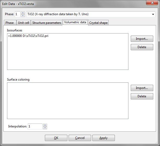
6.4.1 Volumetric data to draw isosurfaces
VESTA enables us to deal with more than two volumetric data sets. Clock [Import...] to select a file in the file selection dialog box. Only files with extensions of supported formats are visible in the file selection dialog box. After selecting a volumetric data file, a Choose operations dialog box appears (Fig. 6.14).
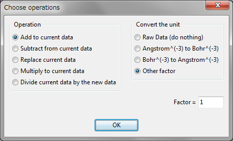
Operation
In the Operation radio box, one of the following five data operations can be selected in addition to conversion of data units.
- “Add to current data”
- “Subtract from current data”
- “Replace current data”
- “Multiply to current data”
- “Divide current data by new data”
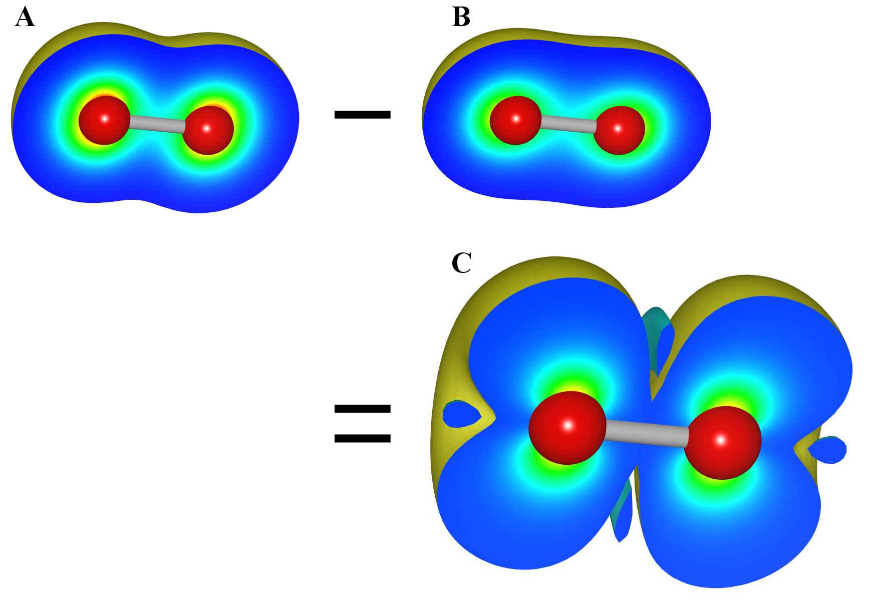
“Multiply to current data” is convenient when squaring wave functions to obtain electron densities (existing probabilities for electrons). The last two options are not displayed when no volumetric data are contained in the current data. In such a case, the first and third options have also the same effect.
Convert the unit
In the Convert the unit radio box, the unit of data can be converted from Å\(^{-3}\) to bohr\(^{-3}\), and vice versa. Select option “Other factor” to multiply the data by an arbitrary factor. Then, click [OK] to import data. Repeating the above procedures allows you to import multiple data, as exemplified in Fig. 6.15.
6.4.2 Volumetric data for surface coloring
Volumetric data for surface coloring can be imported in the same manner as with data for isosurfaces. A typical application of surface coloring is to color isosurfaces of electron densities according to electrostatic potentials.
Interpolation
The spacial resolution of volumetric data can be increased using the algorithm of cubic spline interpolation. The interpolation level is specified in the {Interpolation} text box.
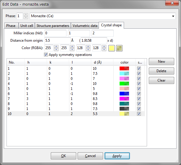
6.5 Crystal Shape
The Crystal Shape tab in the Edit Data dialog box (Fig. 6.16) is used to input and edit the external morphology of crystals. To add a new crystal face, click the [New] button at first, input Miller indices \(hkl\), and the distance from the origin, (0, 0, 0). The distance may be specified in the unit of either its lattice-plane spacing, \(d\), or Å. The color and opacity of the face are specified either as four integers ranging from 0 to 255, or using a color selection dialog box and a slider, which are opened after clicking the square buttons on the right side of the text boxes. When option “Apply symmetry operations” is checked, all the symmetrically equivalent faces are automatically generated.
To delete a face, select an item in the list, and click the [Delete] button or press the \(<\)Delete\(>\) key. Clicking the [Clear] button will delete all the faces in the list.
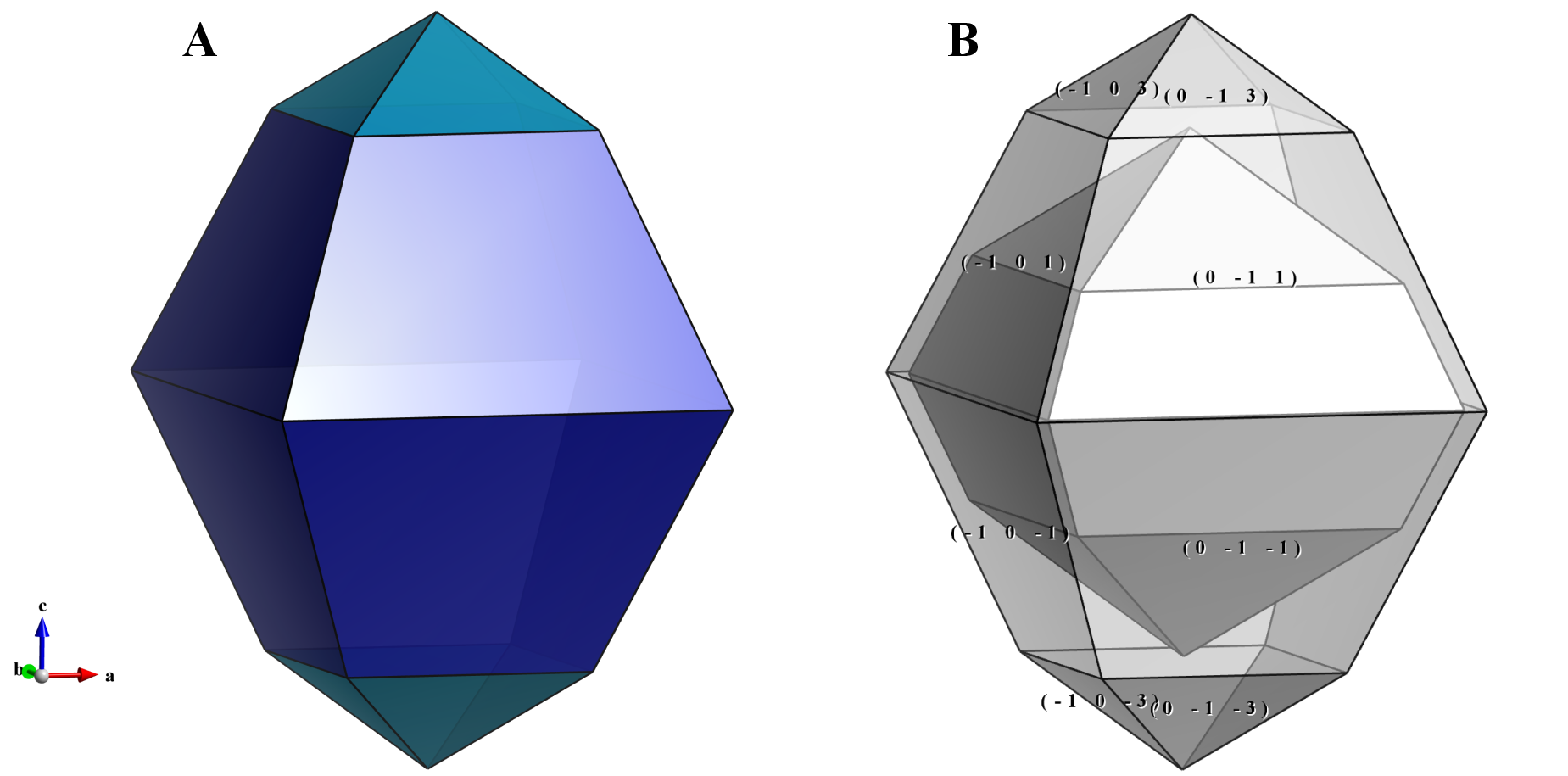
6.5.1 Examples
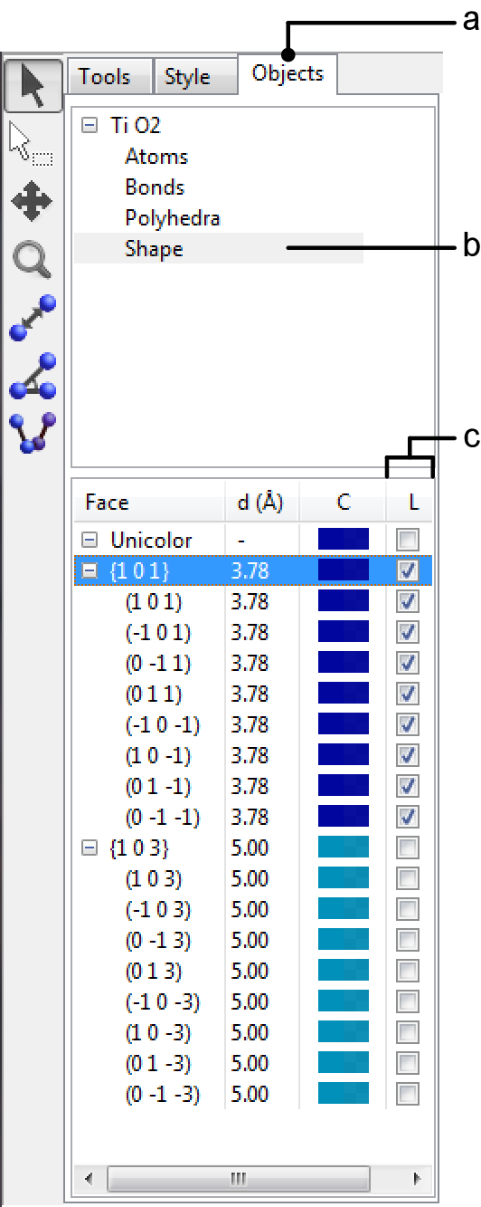
Figure 6.17 shows morphologies of anatase-type TiO\(_2\) crystals composed of {101} and {103} faces. To visualize crystal morphologies, make sure that specified faces compose a closed polyhedron. For example, if only {100} is specified for a tetragonal crystal, it has to form a prismatic shape having an infinite length along the \(c\) axis. In this case, no objects are visible in the Graphics Area.
To adjust relative sizes of faces, edit the distance from the origin to the face. In general, the relative area of the face decreases with increasing distance as Fig. 6.17B illustrates. When the distance of {103} faces is set at a larger value of 5 Å, these faces become smaller with respect to {101} faces. The origin of the crystal shape is just the same as that of a structural model, i.e., a position with the fractional coordinate of (0, 0, 0) is placed at the center of the crystal shape.
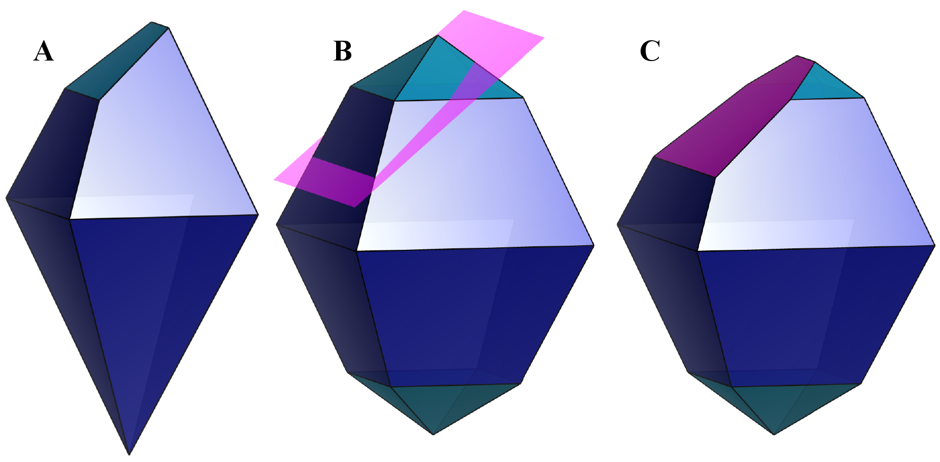
When option “Apply symmetry operations” is unchecked, faces that do not follow space-group symmetry may be inserted (Fig. 6.19A). If multiple faces with the same indices are specified, the face with the smallest distance from the origin is visible (Fig. 6.19B, C). These features make it possbile to represent crystal habits of real crystals.
To display indices of faces as demonstrated in Fig. 6.17B, select the Objects tab in the Side Panel (Fig. 6.18, a), choose “Shape” in the list of phases at the upper half of the page (Fig. 6.18, b), and then click check boxes labeled as “L” (Fig. 6.18, c). See also section 12.2 for the function of the Objects tab.