
Chapter 14
UTILITIES
14.1 Equivalent Positions
The Equivalent Positions dialog box (Fig. 14.1) appears on selection of the “Equivalent Positions...” item under the “Utilities” menu.
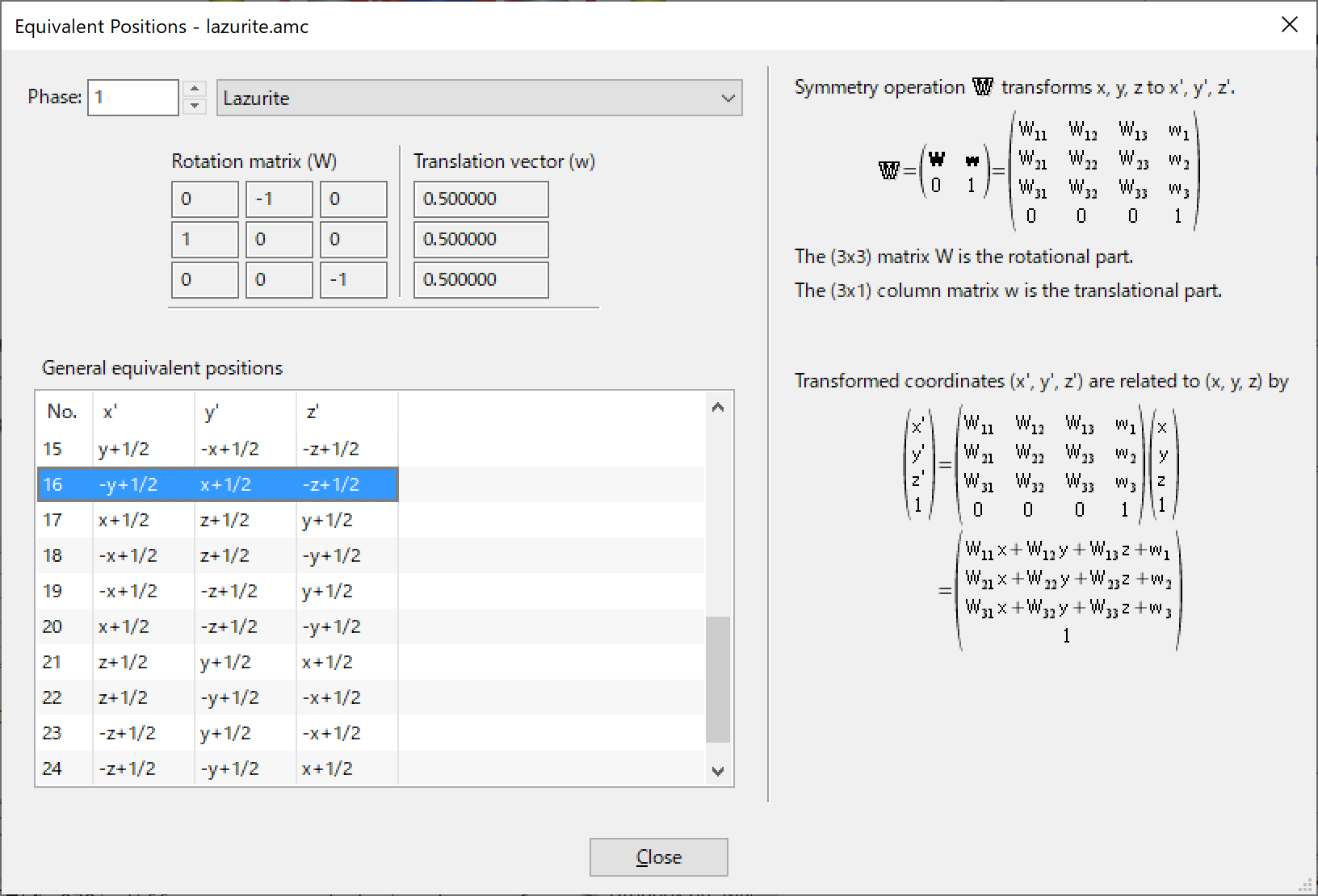
A list of general equivalent positions is displayed in this dialog box. When one of the equivalent positions in the list is selected, the corresponding symmetry operation is displayed in a matrix form at the upper left of the dialog box. In the right side of this dialog box, symmetry operation \(\mathbb {W}\) and transformation of fractional coordinates (\(x\), \(y\), \(z\)) with it are explicitly described (see 6.2.6).
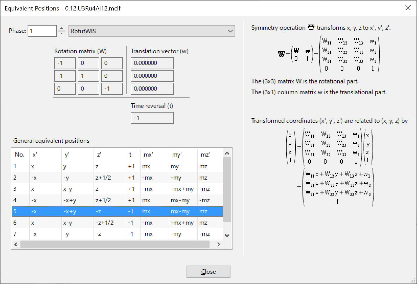
In the case of magnetic space groups, the time reversal term \(t\) and the resultant magnetic moments \(mx\), \(my\), and \(mz\) are also displayed in the list as well as the \(x\), \(y\), \(z\) notation of general positions.
14.2 Geometrical Parameters
This dialog box lists interatomic distances and bond angles recorded in a file *.ffe output by ORFFE [45]. ORFFE calculates geometrical parameters from crystal data in file *.xyz created by RIETAN-FP [12], outputting them in file *.ffe. When reading in input and/or output files of RIETAN-FP (*.ins, *.lst), VESTA also inputs *.ffe automatically provided that *.ffe shares the same folder with *.lst and/or *.ins. Otherwise, *.ffe can be input by clicking the [Read *.ffe] button in the Geometrical Parameters dialog box.
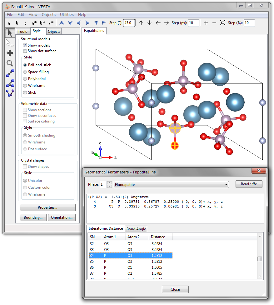
VESTA allows us to locate the bonds and bond angles displayed in the Geometrical Parameters dialog box in the Graphic Area. On selection of a bond (2 atoms) or a bond angle (3 atoms) in this dialog box, the corresponding objects in a ball-and-stick model is selected (highlighted), and vice versa. Thus, atom pairs and triplets associated with geometrical parameters on which restraints are imposed in Rietveld analysis with RIETAN-FP are easily recognized in the ball-and-stick model.
Figure 14.3 exemplifies visualization of a bond in a ball-and-stick model of fluorapatite; a P\(-\)O3 bond (grey line) selected in the dialog box is highlighted in the structural model in the graphic window. The upper part of the dialog box displays detailed information on the P\(-\)O3 bond.
Because ORFFE calculates standard uncertainties of geometrical parameters from both diagonal and off-diagonal terms in the variance-covariance matrix output by RIETAN-FP, the resulting standard uncertaities are more accurate than those evaluated by VESTA from only the diagonal terms. Accordingly, the standard uncertaities output by ORFFE should be described in papers rather than those calculated by VESTA.
14.3 Standardization of Crystal Data
On the use of RIETAN-FP [12], it is highly desirable for an axis setting and fractional coordinates to be standardized in compliance with definite rules [85]. In RIETAN-FP, the following lattice settings are inhibited:
- 1.
- monoclinic system: \(c\)-axis unique setting (\(\gamma \neq 90\)°),
- 2.
- trigonal system: rhombohedral lattice (\(a=b=c\) and \(\alpha = \beta = \gamma \neq 90\)°),
- 3.
- cubic and tetragonal systems: an inversion center not at the origin.
Unless standard settings are adopted, standardization of crystal axes and fractional coordinates is indispensable for Rietveld analysis using RIETAN-FP; otherwise LAZY PULVERIX [86] built in RIETAN-FP fails in generating diffraction indices \(hkl\) and their multiplicities.
Standardized crystal data are generally suitable for structure refinement because atoms in the asymmetric unit are confined in a relatively narrow region. VESTA is capable of launching STRUCTURE TIDY [46] for this purpose.
This feature of standardization of crystal-structure data is particularly useful when searching for compounds with similar structures using the Inorganic Crystal Structure Database (ICSD) [87].
In both STRUCTURE TIDY and LAZY PULVERIX, the following three standard settings are preferred to other settings:
- 1.
- monoclinic system: \(b\)-axis unique setting (\(\beta \neq 90\)°),
- 2.
- trigonal system: hexagonal lattice (\(a = b \ne c\) and \(\gamma = 120\)°),
- 3.
- centrosymmetric space groups: an inversion center at the origin.
Let \(n\) be the number of atoms in the asymmetric unit, and (\(x_j , y_j , z_j\); \(j = 1,2, \cdots , n\)) their fractional coordinates. Then, the standardization parameter, \(\varGamma \), is defined as \begin {equation} \varGamma = \sum _{j=1}^n \Bigl ( x_j^2 + y_j^2 + z_j^2 \Bigr )^{\! \frac {1}{2}} . \end {equation} Note that this equation does not contain occupancies, \(g_j\). STRUCTURE TIDY selects a set of \(x_j\), \(y_j\) and \(z_j\) (\(j = 1,2, \cdots , n\)) minimizing the \(\varGamma \) value. For better distinction between different structure-type branches, STRUCTURE TIDY further outputs another standardization parameter, CG, depending also on lattice parameters: \begin {equation} \begin {split} \mathrm {CG} = &\frac {1}{nV} \left [ \Biggl ( a\sum _{j=1}^n x_j \Biggr )^{\! \! 2} + \Biggl ( b\sum _{j=1}^n y_j \Biggr )^{\! \! 2} + \Biggl ( c\sum _{j=1}^n z_j \Biggr )^{\! \! 2} \right . \\ &\left . + 2ab\cos \gamma \Biggl ( \sum _{j=1}^n x_j y_j \Biggr ) + 2ac\cos \beta \Biggl ( \sum _{j=1}^n x_j z_j \Biggr ) + 2bc\cos \alpha \Biggl ( \sum _{j=1}^n y_j z_j \Biggr ) \right ]^{\! \frac {1}{2}} , \end {split} \end {equation} where \(V\) denotes the unit-cell volume.
VESTA automatically normalize the fractional coordinates between 0 to 1 before standardization of crystal-structure data because the absolute value of each fractional coordinate to be converted by STRUCTURE TIDY should be less than unity; otherwise, the corresponding part of the output text becomes disordered. If lattice parameters and fractional coordinates of atoms in the asymmetric unit are changed on the transformation of the crystal lattice, current crystal data are replaced with the standardized ones. The resulting data are output in the Text Area while standard input and output files of STRUCTURE TIDY are, respectively, saved as data.stin and data.sto in directory tmp under a directory for user settings (see 18.2); data.sto provides us with more detailed information on the standardization of the crystal data.
For example, suppose that a structure data file for Si (space group: \(Fd\bar {3}m\)) is created on the basis of the first setting where Si in the asymmetric unit occupies the 8\(a\) site at (0, 0, 0). Subsequent standardization using STRUCTURE TIDY moves Si from (0, 0, 0) to (1/8, 1/8, 1/8) in such a way that a center of symmetry is present at the origin (second setting). When lattice parameters (\(a\) and \(\alpha \)) and fractional coordinates based on a rhombohedral lattice are input in a trigonal compound, STRUCTURE TIDY converts them into lattice parameters (\(a\) and \(c\)) and fractional coordinates based on a hexagonal lattice.
An example of standardization of crystal data is given below. The structure of a high-\(T_{\mathrm {c}}\) superconductor YBa\(_2\)Cu\(_4\)O\(_8\) is usually represented with the \(c\) axis perpendicular to the CuO\(_2\) conduction sheet and space group Ammm (No. 65) [88]. However, the standard setting described in International Tables for Crystallography, volume A [30] is Cmmm; Rietveld analysis with RIETAN-FP has to be carried out on the basis of Cmmm.
Running STRUCTURE TIDY by selecting the “Standardization of Crystal Data” item under the “Utilities” menus in VESTA, we obtain optimum crystal data based on space group Ammm; they are listed at the tail of data.sto:
Axes changed to : b,c,a

 Setting x,y,z              origin  0.00000 0.00000 0.00000   gamma =   2.9785

 ( 65) C m m m     - j2 i5 c                                 oS30
 -------------------------------------------------------------------------
 DATA   YBa2Cu4O8                                           2.9785  0.7284
 CELL           3.8708 27.2309  3.8402                                   *
 ATOM    O1         4(j)   0        0.05253  1/2                     O2
 ATOM    Ba         4(j)   0        0.36498  1/2                     Ba
 ATOM    Cu1        4(i)   0        0.06138  0                       Cu2
 ATOM    O2         4(i)   0        0.14562  0                       O1
 ATOM    Cu2        4(i)   0        0.21296  0                       Cu1
 ATOM    O3         4(i)   0        0.28178  0                       O4
 ATOM    O4         4(i)   0        0.44786  0                       O3
 ATOM    Y          2(c)   1/2      0        1/2                     Y
 TRANS  b,c,a
 REMARK Transformed from setting  A m m m.
STRUCTURE TIDY converted \(a\), \(b\), and \(c\) axes in Ammm into \(b\), \(c\), and \(a\) axes in Cmmm, respectively. The value of 2.9785 is the standardization parameter ‘gamma’, the last data, 0.7284, in the ‘DATA’ line is CG, and the last data of each site is the site name input by the user.
14.4 Niggli-Reduced Cell
Low-symmetry unit cells can be selected in a variety of ways regardless of the method of determining the unit cell suitable for indexing the whole diffraction pattern. To compare and analyze different indexing solutions, the lattice has to be reduced to a certain unique, peferably standard form, which is usually achieved in the following way [89]:
- In the orthorhombic system, the lattice parameters should be \(a \le b \le c\).
- In the monoclinic system, the lattice parameters should be \(a \le c\) with the \(b\)-axis unique setting.
- In the triclinic system, the reduction becomes more complicated owing to possible multiple choices of basis vectors in the lattice.
Niggli’s approach to unit-cell reduction [89, 90] defines the reduced cell in terms of the shortest vectors: \begin {equation} \nu _1 + \nu _2 + \nu _3 = \mathrm {minimum}. \end {equation} STRUCTURE TIDY [46] transforms the given unit cell to a Niggli-reduced cell to describe the structure in space group \(P1\) or \(P \overline {1}\) when ‘*’ precedes a space-group symbol in an input file. If the Niggli-reduction is successful, the solution is output in the Text Area.
From the reduced form, we can obtain the metric symmetry of the lattice, which is the highest symmetry possible for the lattice on the basis of only geometric considerations. A second application of the Niggli-reduced cell is that different deformation variants of a basis type (arstotype), probably conventionally described with different space groups and probably non-comparable unit cells, can be compared if they have been standardized in their corresponding Niggli-reduced cells.
The output in the Text Area on transformation to a Niggli-reduced cell for a spinel-type oxide CoAl\(_2\)O\(_4\) is given below:
Lattice type        F
Space group name    F d -3 m
Space group number  227
Setting number      1

Lattice parameters

   a        b        c       alpha    beta     gamma
 8.09500  8.09500  8.09500  90.0000  90.0000  90.0000

Unit-cell volume = 530.457520

Structure parameters

                       x          y          z          g        B    Site    Sym.
   1 Co  Co1         0.00000    0.00000    0.00000    1.000    1.000    8a    -43m
====================================================================================

18 atoms, 16 bonds, 0 polyhedra; CPU time = 0 ms

Transformation to a Niggli-reduced cell
====================================================================================
 Setting x,y,z              origin  0.00000 0.00000 0.00000   gamma =   0.2165
 ratio volume Niggli-reduced cell/original cell :  0.25

 (  2) P -1        - i                                       aP2
 -------------------------------------------------------------------------
 DATA                                                       0.2165  0.3437
 CELL           5.7240  5.7240  5.7240    60.000   60.000   60.000       *
 ATOM    Co         2(i)   0.12500  0.12500  0.12500                 Co1
 TRANS  0.5a+0.5b,0.5b+0.5c,0.5a+0.5c
 REMARK Niggli-reduced cell
14.5 Site Potentials and Madelung Energy
VESTA utilizes an external program, MADEL [91], to calculate electrostatic site potentials, \(\phi _i\), and the Madelung energy, \(E_{\mathrm {M}}\), of a crystal. Three methods are used to calculate Madelung energies: Ewald, Evjen, and Fourier methods; the Fourier method is adopted in MADEL. MADEL was originally written by Katsuo Kato (old National Institute for Research in Inorganic Materials) and slightly modified later by one of the authors (F.I.). An advantage of using MADEL in VESTA is that troublesome inputting of formatted data, particularly symmetry operations, is avoidable.
The electrostatic potential, \(\phi _i\), for site \(i\) is computed by \begin {equation} \phi _i = \sum _j \frac {Z_j}{4 \pi \epsilon _0 l_{ij}} , \label {eq:site_potential} \end {equation} where \(Z_j\) is the valence (oxidation state) of the \(j\)th ion in the unit of the elementary charge, \(e\) (\(= 1.602177\)\(\times \)\(10^{-19}\) C), \(\epsilon _0\) is the vacuum permittivity (\(= 8.854188\)\(\times \)\(10^{-12}\) Fm\(^{-1}\)), and \(l_{ij}\) is the distance between ions \(i\) and \(j\); the summation is carried out over all the ions \(j\) (\(i \ne j\)) in the crystal. In case site \(j\) is partially occupied, \(Z_j\) should be multiplied by its occupancy, \(g_j\). \(E_{\mathrm {M}}\) per asymmetric unit is calculated by using the formula \begin {equation} E_\mathrm {M} = \frac {1}{2}\sum _{i} \phi _i Z_i W_i, \label {eq:EM} \end {equation} with \begin {equation} W_i = \frac {\text {(occupncy)} \times \text {(number of equivalent positions)}}{\text {(number of general equivalent positions)}}. \end {equation} The summation in Eq. \eqref{eq:EM} is carried out over all the sites in the asymmetric unit. To obtain the Madelung energy for the unit cell, \(E_M\) must be multiplied by the number of general equivalent positions .
Prior to the execution of MADEL, the oxidation numbers of atoms in the asymmetric unit must be input in the Structure parameters tab of the Edit Data dialog box. Just after launching MADEL, you are prompted to input two parameters, RADIUS and REGION:
| RADIUS: |
Radius of an ionic sphere, s, in Å. The charge-density distribution, \(r\), is given by \begin {equation} \rho (r) = \rho _0 \left [1 - 6(r/s)^2 + 8(r/s)^3 - 3(r/s)^4 \right ], \end {equation} where \(r\) is the distance from the center of the ionic sphere (\(r < s\) and \(\rho (r) = 0\) for \(r \geq s\)). When lines for interstitial sites are not given in the input file, set RADIUS at a value that is large enough but less than the smallest interatomic distance (not half of it!). |
| REGION: |
Reciprocal-space range (in Å\(^{-1}\)) within which Fourier coefficients are summed up. MADEL sums up the Fourier coefficients with respect to all \(hkl\)’s within a sphere having a radius equal to RADIUS. Choose an appropriate value ranging from 2 Å\(^{-1}\) to 4 Å\(^{-1}\) according to the desired precision of calculation. Also, check whether or not a curve for Madelung energy versus REGION is nearly flat around the selected value of REGION. |
The standard output of MADEL is displayed in the Text Area. The unit of \(\phi _i\) is \(e\)/Å (1 \(e\)/Å\(= 14.39965\) V). The accuracy of \(\phi _i\) and \(E_{\mathrm {M}}\) obtained using MADEL is limited to 3 or 4 digits.
The following lines give part of an output file when this feature is applied to investigating distribution of hole carriers in a high-\(T_{\mathrm {c}}\) superconductor, YBa\(_2\)Cu\(_4\)O\(_8\) [88, 92]:
 Potentials of sites in the asymmetric unit

          Charge      W        x        y        z           phi
 Ba       2.000000 0.250000 0.500000 0.135000 0.500000  -1.330304E+00
 Y        3.000000 0.125000 0.500000 0.000000 0.500000  -1.639974E+00
 Cu1      2.000000 0.250000 0.000000 0.213000 0.000000  -2.164424E+00
 Cu2      2.500000 0.250000 0.000000 0.061400 0.000000  -1.798502E+00
 O1      -2.000000 0.250000 0.000000 0.145600 0.000000   1.310975E+00
 O2      -2.000000 0.250000 0.000000 0.052500 0.500000   1.931017E+00
 O3      -2.000000 0.250000 0.500000 0.052100 0.000000   1.925720E+00
 O4      -2.000000 0.250000 0.500000 0.218200 0.000000   1.133873E+00


 Electrostatic energy per asymmetric unit
     -3.318605 e**2/\AA = -47.78676 eV =  -4.610721 MJ/mol
The electrostatic energy per mole is calculated by multiplying a factor of the Avogadro constant (6.02214\(\times \)10\(^{23}\) mol\(^{-1}\)) and \(E_{\mathrm {M}}\) together. In the above calculation, all the holes are assumed to be doped into the Cu2 atoms on the CuO\(_2\) conduction sheet with the Cu1 atoms having an oxidation state of +2.
Standard input files, *.pme, (see p. 385) for MADEL can be output by selecting the Export Data... item under the File menu. This file is helpful in appending fractional coordinates of interstitial sites to obtain their site potentials using the RIETAN-FP–VENUS integrated assistance environment.
14.6 Powder Diffraction Pattern
VESTA utilizes RIETAN-FP [12] to simulate X-ray and neutron powder diffraction patterns from lattice and structure parameters. As described in 16.1, a binary executable file of RIETAN-FP, a graph plotting program, and a template input file, *.ins, for RIETAN-FP are specified in the Preferences dialog box. Setting a variable NMODE at 1 (simulation of a powder diffraction pattern) in the template file is recommended. In addition, change the following data in the template file if necessary:
- Radiation (neutron, characteristic X-ray, or synchrotron X-ray diffraction).
- Wavelength (neutron and synchrotron X-ray diffraction) or target (diffraction using characteristic X rays).
- Geometry (Bragg–Brentano, transmission, or Debye–Scherrer geometry).
- Profile functions and profile parameters.
- Range of diffraction angles: \(2\theta _{\mathrm {min}}\) and \(2\theta _{\mathrm {max}}\).
- Profile cutoff.
Profile parameters refined from typical diffraction data measured on a powder diffractometer, which is often used on a routine basis, are preferable to those in one of template files included in the distribution files of the RIETAN-FP–VENUS system. Further, a variable, NPAT, must be given in the template file to specify a graph plotting program:
- 1.
- NPAT = 1: a pair of files, *.plt including commands to plot a graph and *.gpd storing data to be graphed, for gnuplot1 (default),
- 2.
- NPAT = 2: an Igor text file, *.itx, for Igor Pro2 or WinPLOTR,3
- 3.
- NPAT = 3: a text file, *.itx, for RietPlot.4
The use of gnuplot is highly recommended because it is free software supporting many features; commands may be modified and added in *.plt to change the appearance of a graph. For details in the content of *.plt, refer to RIETAN-FP_manual.pdf. If NPAT = 1, no graph plotting program need to be specified in the Preferences dialog box.
Stable versions of gnuplot are included in the distribution files of the RIETAN-FP–VENUS system5 for Windows and macOS.
Gnuplot can output a PDF file, *.pdf, whose margins are automatically cut, which is very convenient when exporting the resulting PDF file to an application such as TE X, Microsoft PowerPoint and Word, and Adobe Illustrator. (Windows) or ps2pdf (macOS).
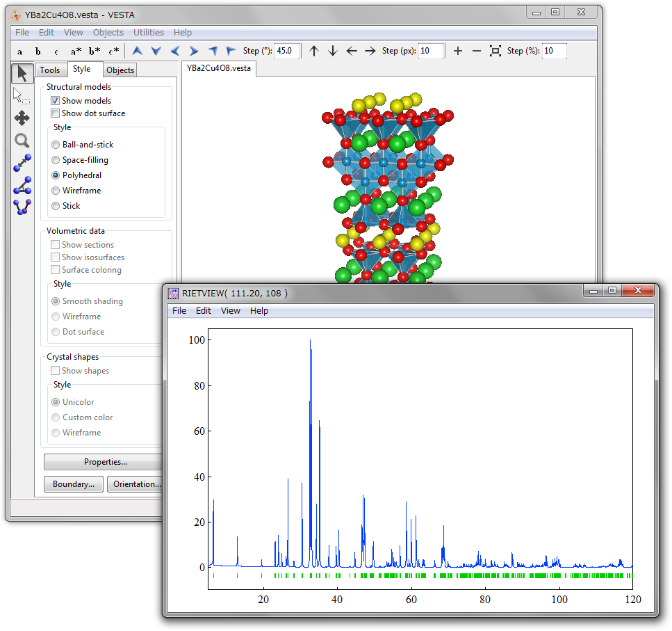
On selection of the “Powder Diffraction Pattern...” item under the “Utilities” menu, a series of procedures, i.e., (a) generation of an input file, *.ins, for RIETAN-FP, (b) execution of RIETAN-FP in the simulation mode (NMODE = 1), and (c) representation of the resulting text file(s) by a graphing program are executed by VESTA as if the two programs were implemented in VESTA (Fig. 14.4). Text files, *.ins, *.lst (standard output), and a pair of files (*.plt and *.gpd for gnuplot) or *.itx, output by RIETAN-FP are saved in folder tmp under the settings directory (see 18.2).
For those who have not any program to plot data in *.itx with the Igor text format, a small Java program named PowderPlot,6 which was developed by one of the authors (K.M.), is included in the archive file of VESTA.
VESTA automatically standardizes lattice settings when outputting *.ins to satisfy conditions required by LAZY PULVERIX [86], which is embedded in RIETAN-FP to generate diffraction indices, \(hkl\), and their multiplicities, \(m\). Standard lattice settings adopted in LAZY PULVERIX are just the same as those in STRUCTURE TIDY (see 14.3) [85, 46]: second settings in centrosymmetric space groups with more than one origin choice and first settings in the other space groups. Then, beware that diffraction indices displayed in PowderPlot are incompatible with the coordinate system adopted in VESTA if the lattice setting in VESTA is other than a standard one.
A list of reflections output at the tail of *.lst if NPRINT \(>\) 0 provides us with a variety of information about \(hkl\) reflections included in a \(2\theta \) range specified by the user. For instance, simulation of an X-ray diffraction pattern for fluorapatite gives the following output where line heads were deleted for convenience:
  h    k    l  Code     2-theta          d     Ical |F(crys)| |F(magn)|     POF      FWHM    m       Dd/d
  1    0    0    +1      10.895    8.11382    12287   16.7800      -      1.001   0.07451    6   0.013637
  1    0    0    +2      10.923    8.11382     6113   16.7800      -      1.001   0.07451    6   0.013602
  1    0    1    +1      16.877    5.24919     4465   11.1545      -      0.999   0.07443   12   0.008757
  1    0    1    +2      16.919    5.24919     2221   11.1545      -      0.999   0.07443   12   0.008734
  1    1    0    +1      18.929    4.68452     2079   12.0931      -      1.001   0.07445    6   0.007795
  1    1    0    +2      18.976    4.68452     1034   12.0931      -      1.001   0.07445    6   0.007775
  2    0    0    +1      21.891    4.05691     9679   30.2953      -      1.001   0.07453    6   0.006726
  2    0    0    +2      21.946    4.05691     4814   30.2953      -      1.001   0.07453    6   0.006709
  1    1    1    +1      22.945    3.87283     8580   21.1855      -      1.000   0.07457   12   0.006413
  1    1    1    +2      23.003    3.87283     4268   21.1855      -      1.000   0.07458   12   0.006397
   .....
where Code +1 and Code +2 are, respectively, \(K\alpha _1\) and \(K\alpha _2\) reflections (‘+’ means not \(\overline {h}\overline {k}\overline {l}\) but \(hkl\) reflection in Friedel pairs), 2-theta is the diffraction angle \(2\theta \), d is the lattice-plane spacing, Ical is the calculated integrated intensity adjusted in such a way that the strongest reflection has an intensity of \(10^5\), F(nucl) and F(magn) are, respectively, the crystal-structure and magnetic-structure factors, POF is the preferred-orientation function, FWHM is the full-width at the half-maximum intensity, m is the multiplicity, and Dd/d is the resolution, \(\Delta d / d\).
14.7 Structure Factors
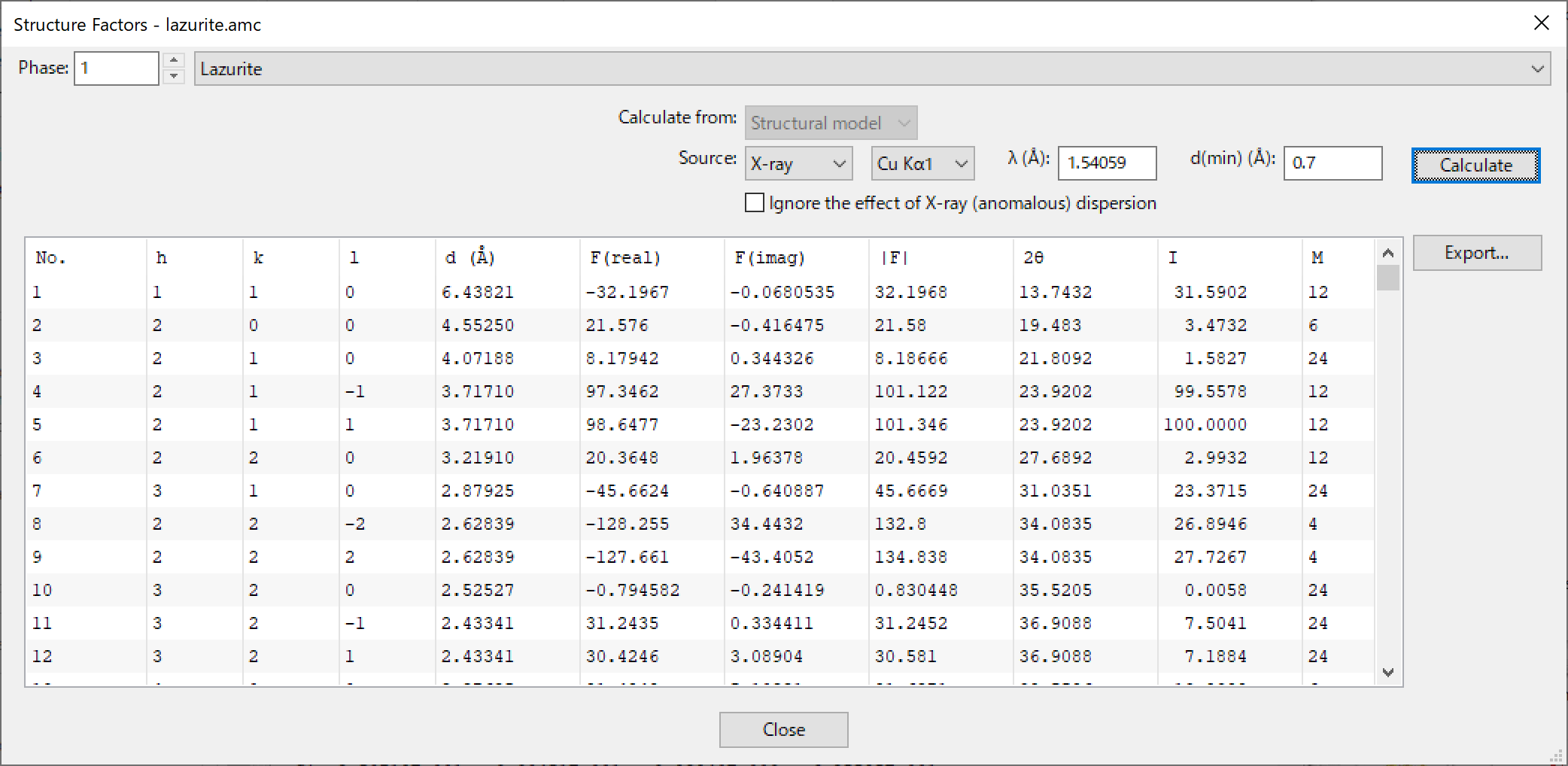
Selection of “Utilities” menu \(\Rightarrow \) “Structure Factors...” pops up the Equivalent Positions dialog box (Fig. 14.5), whose use makes it possible to calculate structure factors from structural models (structure parameters) or volumetric data (electron or coherent-scattering length densities, \(\rho \)).
If multiple phase data are included in the data set, select a phase, for which structure factors are calculated, at the top of the dialog box. If the phase data contain both structural and volumetric data, select {Structural model} or {Volumetric data} in the list box to specify the type of data from which structure factors are calculated. In the Source list box, {X-ray} and {Neutron} beam sources can be switched, and some typical characteristic X-rays can be selected at a list box next to the Source list box. For the neutron source and the X-ray source with its target specified as {Custom}, the wavelength can be edited in the text box. The minimum lattice-plane spacing, \(d\), of reflections whose structure factors are calculated is also specified in the text box.
In X-ray diffraction, structure factor \(F\) of reflection \(\bm {h}\) with diffraction indices \(hkl\) is formulated as \begin {equation} F(\bm {h}) = \sum _{j=1}^n g_j f_{j} (\bm {h}) T_j (\bm {h}) \exp \bigl [ 2\pi \mathrm {i} \big ( hx_j + ky_j + lz_j \big ) \bigr ], \label {eq:structure-factor-Xray} \end {equation} where \(j\) is the atom number, \(n\) is the total number of atoms in the unit cell, \(g_j\) is the occupancy, \(f_{j} (\bm {h})\) is the (X-ray) atomic form factor, \(T_j (\bm {h})\) is the Debye–Waller factor, and \(x_j\), \(y_j\), and \(z_j\) are the fractional coordinates. The atomic form factor \(f(\bm {h})\) is a complex number that can be divided into four separate components as \begin {equation} f(\bm {h}) = f_{0} (\bm {h}) + f^\prime + \mathrm {i} f^{\prime \prime } + f_\mathrm {NT}, \end {equation} where \(f_{0} (\bm {h})\) is the coherent scattering factor, \(f^\prime \) and \(f^{\prime \prime }\) are the real and imaginary components of the dispersion correction, and \(f_{\mathrm {NT}}\) is the nuclear Thomson scattering [93],. The coherent atomic scattering factor \(f_0\), which is a function of \(\sin \theta / \lambda \), is usually analytically approximated by a sum of exponentials plus a constant: \begin {equation} f_0 (\sin \theta / \lambda ) = \sum _{i=1}^N a_i \exp \left ( −b_i \frac {\sin ^2 \theta }{ \lambda ^2} \right ) + c. \end {equation} VESTA utilizes a set of parameters (\(a_i\), \(b_i\), and \(c\)) with \(N=5\) tabulated in [94]. These parameters can be used in the range of \(0 < \sin \theta / \lambda < 6\). The real and imaginary parts, \(f^\prime \) and \(f^{\prime \prime }\), of the dispersion correction are calculated by linear interpolation of theoretically calculated form factors in energy ranges of \(E=1\)–\(10\) eV and \(E=0.4\)–\(1.0\) MeV [95, 96]. The nuclear Thompson scattering term \(f_{\mathrm {NT}}\) is small and negative in the phase relative to the electronic form factor, with small (negligible) dependences on \(\lambda \) and \(\sin \theta / \lambda \).
In the case of neutron diffraction, \(f_j (\bm {h})\) has to be replaced by the coherent-scattering length [10], \(b_{\mathrm {c}}\): \begin {equation} F(\bm {h}) = \sum _{j=1}^n g_j b_{\mathrm {c}j} T_j (\bm {h}) \exp \bigl [ 2\pi \mathrm {i} \big ( hx_j + ky_j + lz_j \big ) \bigr ] . \label {eq:structure-factor-neutron} \end {equation} The value of \(b_{\mathrm {c}}\) is constant regardless of \(\bm {h}\) because scattering of neutrons by negligibly small atomic nuclei does not depend on \(\sin \theta / \lambda \) (in the absence of magnetic atoms).
On calculation of structure factors from structural models, \(a_i\), \(b_i\), \(c_i\), \(b_{\mathrm {c}}\), \(f^\prime \), \(f^{\prime \prime }\), \(f_{\mathrm {NT}}\), and the mass attenuation coefficient, \(\mu / \rho \) (\(\mu \): linear attenuation coefficient, \(\rho \): density), of each element are output in the Text Area as follows:
         a1         a2         a3         a4         a5         c
         b1         b2         b3         b4         b5         bc
  Cu: 14.014192   4.784577   5.056806   1.457971   6.932996  -3.254477
       3.738280   0.003744  13.034982  72.554793   0.265666   7.718000
  Se: 17.354071   4.653248   4.259489   4.136455   6.749163  -3.160982
       2.349787   0.002550  15.579460  45.181201   0.177432   7.970000
   O:  2.960427   2.508818   0.637853   0.722838   1.142756   0.027014
      14.182259   5.936858   0.112726  34.958481   0.390240   5.803000

X-ray dispersion coefficients for  = 0.154059 nm
       f’             f’’            f_NT           / (cm^2/g)
  Cu: -2.02777E+00,   5.83511E-01,  -7.26020E-03,   5.01091E+01
  Se: -7.87865E-01,   1.13462E+00,  -8.03140E-03,   7.75653E+01
   O:  4.77543E-02,   3.20501E-02,  -2.19440E-03,   1.09804E+01
If all the parameters of some elements are 0, the element names are not recognized by the program; consequently, such elements do not contribute to calculated structure factors at all. The element names can be edited in the Structure parameters page of the Edit Data dialog box. When an option of “Ignore the effect of X-ray (anomalous) dispersion” is enabled, \(f^\prime \), \(f^{\prime \prime }\), and \(f_{\mathrm {NT}}\) are set at 0, and none of these values are output in the Text Area.
Structure factors, \(F(\bm {h})\), can be calculated by the Fourier transform of \(\rho (x, y, z)\): \begin {equation} F(\bm {h}) = \iiint \rho (x, y, z) \exp [2\pi \mathrm {i} (hx + ky + lz)] \mathrm {d}x\mathrm {d}y\mathrm {d}z. \label {eq:structure-factor-Vol1} \end {equation} In the {Volumetric data} mode, Eq. \eqref{eq:structure-factor-Vol1} is approximated by numerical integration of discrete densities: \begin {equation} F(\bm {h}) = \sum _{x=0}^1 \sum _{y=0}^1 \sum _{z=0}^1 \rho (x, y, z) \mathrm {d}V \exp [2\pi \mathrm {i} (hx + ky + lz)] . \end {equation} In this mode, only the minimum \(d\) value can be specified, and no other options affect calculation results.
14.8 Fourier Synthesis
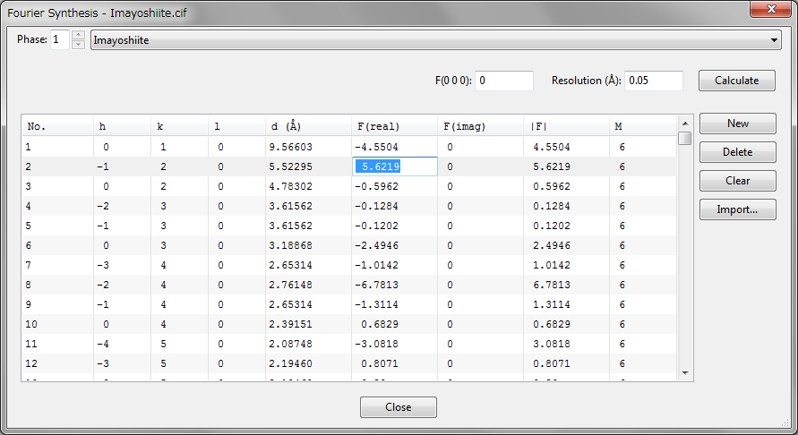
On selection of “Utilities” menu \(\Rightarrow \) “Fourier Synthesis...”, structure factors can be imported from an external file to carry out Fourier synthesis from them to visualize one of observed, calculated, or difference densities. Prior to the use of this menu, lattice parameters and space-group symmetry have to be given. The Fourier Synthesis dialog box is used to import and edit structure factors (Fig. 14.6). To import structure factors, click the [Import...] button. One of observed, calculated, or difference structure factors (\(F_{\mathrm {o}}\), \(F_{\mathrm {c}}\), or \(F_{\mathrm {o}}-F_{\mathrm {c}}\)) can be imported from *.fcf files output by SHELX-97 [97] with a “LIST 3” command. \(F_{\mathrm {o}}\) can also be imported from input files, *.mem and *.fos, for MEM analysis [7, 8, 9]. To import structure factors from files with formats other than the above ones, create a text file where each line contains the following data in free format:
h k l |Fo| |Fc| Fc(real) Fc(imag) sigma(F)
Only unique reflections should be given in the file because all the equivalent reflections are automatically generated according to the current space group. If parts of reflections in the list do not satisfy conditions limiting possible reflections in the space group, a warning message will appear, and their structure factors will be reset to 0. \(F(0 0 0)\) is separately input in the text box placed above the list of structure factors. In addition, the spacial resolution in real space must be specified in the unit of Å. After all the data have been input, press the [Calculate] button to carry out Fourier synthesis from them.
14.9 Model Electron Densities
On selection of the “Utilities” menu \(\Rightarrow \) “Model Electron Densities”, electron densities are calculated by the Fourier transform of structure factors, \(F(\bm {h})\), that are calculated from structure parameters and atomic scattering factors of free atoms [94] with Eq. \eqref{eq:structure-factor-Xray}. The spacial resolution of electron densities is specified in the unit of Å. The number of grids along each crystallographic axis, \(N_x\), is automatically set such that \(N_x\) gives a resolution close to the specified value and that \(N_x\) satisfies symmetrical constraints. Then, the electron density, \(\rho (x,y,z)\), at the coordinates of \((x, y, z)\) is calculated by \begin {equation} \rho (x, y, z) = \frac {1}{V} \sum _{h=\frac {-N_x}{2}}^{\frac {N_x}{2}} \sum _{k=\frac {-N_y}{2}}^{\frac {N_y}{2}} \sum _{l=\frac {-N_z}{2}}^{\frac {N_z}{2}} F(\bm {h}) \exp [-2\pi \mathrm {i} (hx + ky + lz)] . \end {equation} If the resolution is not sufficiently high, spurious noises appear in the resulting densities because of the so-called termination effect in Fourier synthesis. On the other hand, atomic scattering factors compiled in Ref. [94] are reliable only in a range of \(\sin \theta / \lambda < 6 \; \mathrm {\AA }^{-1}\), which corresponds to a spacial resolution of approximately 0.042 Å. VESTA simply extrapolates the atomic scattering factors given in Ref. [94] even when the specified resolution is smaller than 0.042 Å.
14.10 Model Nuclear Densities
On selection of the “Utilities” menu \(\Rightarrow \) “Model Nuclear Densities”, densities of coherent-scattering lengths [10], \(b_{\mathrm {c}}\), are calculated by the Fourier transform of structure factors, \(F(\bm {h})\), that are calculated from structure parameters and \(b_{\mathrm {c}}\)’s of atoms with Eq. \eqref{eq:structure-factor-neutron}. The spacial resolution is set in the same manner as with the calculation of model electron densities (see section 14.9).
14.11 Patterson Densities
On selection of the “Utilities” menu \(\Rightarrow \) “Patterson Densities”, Patterson functions in the unit cell are calculated in three different modes:
- 1.
- “From Model Electron Densities” submenu: from structure parameters and atomic scattering factors of free atoms [94].
- 2.
- “From Model Nuclear Densities” submenu: from structure parameters and coherent-scattering lengths of atoms.
- 3.
- “From Volumetric Data” submenu: by convolution of volumetric data that are currently displayed.
On selection of the first two submenu, structure factors are calculated with Eqs. \eqref{eq:structure-factor-Xray} and \eqref{eq:structure-factor-neutron}, respectively, with the spacial resolution of electron or coherent-scattering-length densities specified in the unit of Å. Then, the Patterson density, \(P(x,y,z)\), at the coordinates of \((x, y, z)\) is calculated by \begin {equation} P(x, y, z) = \frac {1}{V} \sum _{h=\frac {-N_x}{2}}^{\frac {N_x}{2}} \sum _{k=\frac {-N_y}{2}}^{\frac {N_y}{2}} \sum _{l=\frac {-N_z}{2}}^{\frac {N_z}{2}} |F(\bm {h})|^2 \exp [-2\pi \mathrm {i} (hx + ky + lz)] , \label {eq:patterson} \end {equation} where \(N_x\), \(N_y\), and \(N_z\) are the numbers of grids along the \(x\), \(y\), and \(z\) axes, respectively (see section 14.9).
When Patterson functions are calculated from the current volumetric data, structure factors are calculated by \begin {equation} F(h,k,l) = \sum _x \sum _y \sum _z \rho (x, y, z) \exp [2\pi \mathrm {i} (hx + ky + lz)], \end {equation} and then \(P(x,y,z)\) is computed by Eq. \eqref{eq:patterson}. Therefore, the spacial resolution of the Patterson function is the same as that of the volumetric data.
14.12 2D Data Display
We sometimes wish to visualize 2D distribution of a physical quantity on a plane. In such a case, open the 2D Data Display window to display 2D images of volumetric data. Details in the feature of 2D Data Display are described in chapter 15.
14.13 Line Profile
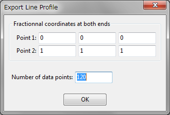
Numerical values on a line segment with an equal step are calculated from volumetric data by linear interpolation of volumetric data and output in a text file to plot a line profile by a graphing program such as Igor Pro, gnuplot, and WinPLOTR. After this item has been selected, a dialog box (right figure) is opened to input fractional coordinates, (\(x\), \(y\), \(z\)), of both ends and the total number of data points to be calculated. After clicking the [OK] button, a file selection dialog box appears and prompts you to input the name of an output file.
The top part of an output file when dealing with electron densities in rutile-type TiO\(_2\) is listed below:
TiO2 (rutile)
Point 1:  0.00000  0.00000  0.00000
Point 2:  0.30530  0.30530  0.00000
50
 0.000000E+000  2.899010E+002
 4.047903E-002  2.582953E+002
 8.095806E-002  2.272991E+002
 1.214371E-001  1.836505E+002
 1.619161E-001  1.328268E+002
 .....
The first line gives a title, followed by two lines for the fractional coordinates of both ends, those of Ti and O atoms in this case. The fourth line is the total number of data points (= 50), followed by 50 lines. In each of the 50 lines, the first and second columns give a distance from “Point 1” in the unit of Å and an interpolated value, respectively.
14.14 Peak Search
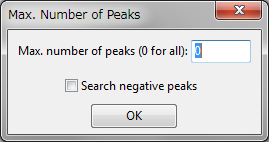
To search for peak positions in volumetric data, choose “Peak Search” under the “Utilities” menu. When this item is selected, a dialog box (right figure) is opened to restrict the maximum number of peaks listed in the Text Area. Enter 0 to list all the peaks detected in the volumetric data. The following data are listed in the Text Area: integrated value of volumetric data, number of peaks, peak positions, peak values, integrated value of volumetric data for each peak, and Voronoi volume [21] calculated for each peak.
Results of peak search for electron densities in the unit cell of rutile-type TiO\(_2\) are exemplified below:
Integrated value of volumetric data over the unit cell: 75.999979, 0.000000

Number of peaks in the volumetric data = 10
Number of voxels at Voronoi boundaries = 60870/262144
            x         y         z     Peak value     Integrated         Volume
  1   0.00000   0.00000   0.00000    2.89901E+02    1.99855E+01    7.64201E+00
  2   0.50000   0.50000   0.50000    2.89901E+02    1.99855E+01    7.64201E+00
  3   0.29688   0.29688   0.00000    5.66020E+01    9.00724E+00    1.17901E+01
  4   0.70312   0.70312   0.00000    5.66020E+01    9.00724E+00    1.17901E+01
  5   0.79688   0.20312   0.50000    5.66020E+01    9.00724E+00    1.17901E+01
  6   0.20312   0.79688   0.50000    5.66020E+01    9.00724E+00    1.17901E+01
The integrated values represent numbers of electrons per each site, which is calculated by summation of numbers of electrons over the Voronoi volume of the site.
14.15 Conversion of Electron Densities
We can extract some important physical quantities from electron densities obtained experimentally from X-ray diffraction experiments. Let \(\rho (\bm {r})\) be the electron density at the position vector \(\bm {r}\), and \(\nabla \rho (\bm {r})\) the gradient vector field of \(\rho (\bm {r})\). With VESTA, we can calculate Laplacians of electron densities \(\nabla ^2 \rho (\bm {r})\), electronic kinetic-energy densities \(g(\bm {r})\), electronic potential-energy densities \(\nu (\bm {r})\), and electronic energy densities \(h_{\mathrm {e}}(\bm {r})\) from electron densities displayed in the current page according to Tsirelson’s procedures [48]. Consideration of these functions, particularly \(\nabla ^2 \rho (\bm {r})\) and \(h_{\mathrm {e}}(\bm {r})\), is not restricted by the bond critical point, \(\bm {r}_{\mathrm {b}}\), where \(\nabla \rho (\bm {r}) = 0\), providing us with a comprehensive characterization of chemical bonding in molecules and crystals.
The electronic kinetic-energy density is expressed as \begin {equation} g(\bm {r}) = \frac {\hbar ^2}{m} \left \{ \frac {3}{10} \left ( 3 \pi ^2 \right )^{2/3} \bigl [ \rho (\bm {r}) \bigr ]^{5/3} + \frac {\lambda \bigl [ \nabla \rho (\bm {r}) \bigr ]^2 }{\rho (\bm {r})} + \frac {k \nabla ^2 \rho (\bm {r})}{2} \right \}, \end {equation} where \(\hbar ^2\) is Dirac’s constant, and \(m\) is the electron mass; the gradient \(\hbar \)-expansion of the Green function around the classical Thomas-Fermi approximation [98] yields \(\lambda \) = 1/72 and \(k\) = 1/6. The electronic-energy density equals the sum of \(g(\bm {r})\) and \(\nu (\bm {r})\): \begin {equation} h_\mathrm {e}(\bm {r}) = g(\bm {r}) + \nu (\bm {r}) \end {equation} with \begin {equation} \nu (\bm {r}) = \frac {\hbar ^2}{4m} \nabla ^2 \rho (\bm {r}) - 2g(\bm {r}). \end {equation}
The electronic-energy density at \(\bm {r}_{\mathrm {b}}\) gives a straightforward criterion for the recognition of the atomic interaction type. That is, \(h_{\mathrm {e}}(\bm {r}) < 0\) is observed in shared-type atomic interactions whereas \(h_{\mathrm {e}}(\bm {r}) > 0\) is observed in closed-shell interactions. In a similar manner, if the electrons are locally concentrated around \(\bm {r}_{\mathrm {b}}\) \([\nabla ^2 \rho (\bm {r}_{\mathrm {b}}) < 0]\), the electrons are shared by both nuclei, which is typical for shared or covalent atomic interactions. Otherwise the electrons are concentrated in each of the atomic basins \([\nabla ^2 \rho (\bm {r}_{\mathrm {b}}) > 0]\), and the atomic interaction belongs to the closed-shell type.
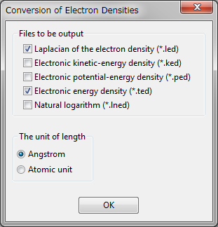
On selection of the “Conversion of Electron Densities” item in the “Utilities” menu, a dialog box appears (right figure) to specify files to be output. The user-selected files are output in the general volumetric-data format (see p. 379) to either a directory where the electron densities are recorded or a directory specified by the user if VESTA fails in writing the files under that directory. By default, files storing volumetric data of \(\nabla ^2 \rho (\bm {r})\) and \(h_{\mathrm {e}}(\bm {r})\) are, respectively, output to files *.led and *.ted with their contents visualized in two pages.
The unit of input data should also be specified: either angstrom (Å\(^{-3}\)) or atomic unit (\(a_0^{-3}\)). Table 14.1 lists units of output data.
| Input data |
Output data
|
||||
|
\(\nabla ^2 \rho (\bm {r})\) |
\(g(\bm {r})\) |
\(\nu (\bm {r})\) |
\(h_{\mathrm {e}}(\bm {r})\) |
||
|
|
|
|
|
|
|
| Å\(^{-3}\) |
Å\(^{-5}\) |
\(E_{\mathrm {h}}a_0^{-3}\) |
\(E_{\mathrm {h}}a_0^{-3}\) |
\(E_{\mathrm {h}}a_0^{-3}\) |
|
| \(a_0^{-3}\) |
\(a_0^{-5}\) |
\(E_{\mathrm {h}}a_0^{-3}\) |
\(E_{\mathrm {h}}a_0^{-3}\) |
\(E_{\mathrm {h}}a_0^{-3}\) |
|
