Chapter 11
INTERACTIVE MANIPULATIONS
11.1 Rotate
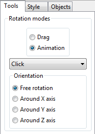
In the Rotation mode, mouse behavior can be changed after clicking the Tools tab in the Side Panel (Fig. 11.1).
11.1.1 Drag mode
In the “Drag” mode, drag the mouse while pressing the left mouse button to rotate objects in the Graphics Area. The objects are rotated while dragging with the mouse. They are never rotated after releasing the mouse button. In the [Free rotation] mode, the rotation axis becomes normal to the direction along which the mouse is moved. To restrict the rotation axis, select [Around X axis], [Around Y axis], or [Around Z axis] in the pull-down menu of the Rotation modes frame box.
11.1.2 Animation mode
Three types of animation modes can be used in VESTA: “Click”, “Push”, and “Random” modes. The step width of rotation (in degrees/frame) and intervals between frames (in ms) are specified in the Preferences dialog box (see chapter 16).
“Click” mode
In the “Click” mode, click the left mouse button to rotate the objects. In the “Click” plus [Free] rotation modes, the rotation axis is perpendicular to a line connecting the clicked position and the central point. To restrict the rotation axis, select [Around X axis], [Around Y axis], or [Around Z axis] in the pull down menu of the Rotation modes frame box. To stop rotating the objects, select either the “Drag” or “Push” mode. The animation speed (intervals between frames in ms) is specified in the Preferences dialog box.
“Push” mode
In the “Push” mode, press the left mouse button at point 1 and drag the mouse to point 2. In the [Free rotation] mode, objects are rotated around an axis perpendicular to a line connecting points 1 and 2. The rotation speed is proportional to the speed of moving the mouse. The objects stop rotating immediately after releasing the left mouse button. To restrict the rotation axis, select [Around X axis], [Around Y axis], or [Around Z axis] in the pull down menu of the Rotation modes frame box.
“Random” mode
In the “Random” mode, the rotation axis is automatically set and it changes dynamically. To stop the rotation of the objects, select either the “Drag” or “Push” mode.
11.2 Magnify
Objects are magnified in proportion to the distance of dragging the mouse upward. On the other hand, they are shrunk in inverse proportion to the distance of dragging the mouse downward.
11.3 Translate
Drag the mouse in the Graphics Area to translate objects. When a lattice plane with a color specified in the Lattice Planes dialog box is selected and dragged in this mode, it is interactively moved. Otherwise the entire objects are translated with the mouse along the same direction.
11.4 Select
Several ways of selecting objects can be used. On the use of the select mode in the Vertical Toolbar, left click on an object to select it. To select all the objects in a certain area, press the left mouse button and drag the mouse to specify an area. On selection of new objects, objects that have previously been selected are reset to the normal state. To select additional objects while keeping the present objects alive, press \(<\)Shift\(>\) while clicking or dragging the Graphics Area. Regardless of the current manipulation mode, two or more objects can be selected by clicking or dragging on them while pressing the \(<\)Shift\(>\) key. A single object is selectable by double-clicking on it. Objects other than atoms, bonds, and polyhedra cannot be selected. For example, atoms behind isosurfaces can be selected.
After a single object has been selected, a variety of information about it is output in the Text Area. The estimated standard uncertainty is also displayed for interatomic distance, bond angle, and dihedral angle if those of lattice parameters and fractional coordinates have been supplied. However, note that VESTA gives only rough estimates of standard uncertainties by neglecting off-diagonal elements of the variance-covariance matrix because no off-diagonal elements are included in crystal-data files.
Objects can also be selected by using the Objects tab in the Side Panel (see section 12.2), the Vectors dialog box (see section 11.4), and the Geometrical Parameters dialog box (see section 14.2).
Press the \(<\)Delete\(>\) key to hide selected objects. The hidden objects are not actually deleted but just made invisible. To restore all the hidden objects, press the \(<\)Esc\(>\) key. By hiding part of coordination polyhedra, you can easily mix polyhedra with a ball-and-stick model.
11.4.1 Atom
On selection of an atom, site number, site name, symbol of the element, fractional coordinates \((x, y, z)\), translation vector, symmetry operations (coordinate triplet), occupancy, isotropic atomic displacement parameter, site multiplicity plus Wyckoff symbol, and site symmetry are displayed for the atom. For example, selection of Al and O atoms connected with each other in a ball-and-stick model of \(\alpha \)-Al\(_2\)O\(_3\) gives the following lines:
Atom:  1    Al Al  0.00000  1.00000 -0.15000  ( 0, 1,-1)+ -y, -x, z+1/2
            Occ. = 1.000       Ueq = 0.17370     12c      3.
Atom:  2     O  O  0.33333  0.97667 -0.08333  ( 0, 0,-1)+ -y+1/3, x-y+2/3, z+2/3
            Occ. = 1.000       Ueq = 0.19915     18e      .2
When atoms are rendered as displacement ellipsoids, information about principal axes and mean square displacements are also output:
Atom:  2     O  O  0.97667  0.64333  0.08333  ( 0, 0, 0)+ x-y+2/3, x+1/3, -z+1/3
            Occ. = 1.000       Ueq = 0.19915     18e      .2

Principal axes of the anisotropic atomic displacement parameters
        MSD (Å^2)      x         y         z            u         v         w
  1     0.003223    -0.043986  0.027435 -0.023150    -0.005924  0.006668 -0.001785
  2     0.002471     0.027516  0.041255 -0.003390     0.010805  0.010027 -0.000261
  3     0.001873    -0.013219  0.012054  0.039403    -0.001318  0.002930  0.003038
11.4.2 Bond
When a bond is selected, its length is displayed with its estimated standard uncertainty, if any, in the Text Area as well as the Status Bar. Site number, site name, symbol of the element, fractional coordinates \((x, y, z)\), translation vector, and symmetry operations are also displayed for two atoms connected with the bond. For example, on selection of an Al\(-\)O bond in the ball-and-stick model of \(\alpha \)-Al\(_2\)O\(_3\), the following three lines are output:
Bond: l(Al-O) =  1.96249(0) Angstrom
   1      Al Al  1.00000  0.00000  0.15000 ( 1, 0, 0)+ y, x, -z+1/2
   2       O  O  1.00000  0.31000  0.25000 ( 1, 0, 0)+ -y, x-y, z
11.4.3 Coordination polyhedron
When a coordination polyhedron with a coordination number of \(n\) is selected, information on the central atom and coordinating atoms (ligands), distances between the central atom and coordinating atoms are listed in the Text Area. Further, geometric information described below is displayed in the Text Area; the polyhedral volume, \(D\), \(<\!\! \lambda \!\! >\), and \(\sigma ^2\) are useful when investigating structural changes under high/low temperature and high pressure [67].
Polyhedral volume
The volume of the selected coordination polyhedron is calculated as a fundamentally important physical quantity [31]. For example, distortion in perovskite-type compounds, ABO\(_3\) can be quantified with polyhedral volume ratios, \(V_A / V_B\), rather than with tilting angles [68].
Distortion index
A distortion index, \(D\), based on bond lengths was defined by Baur [32] as \begin {equation} D = \frac {1}{n} \sum _{i=1}^n \frac {\vert l_i - l_\mathrm {av} \vert }{l_\mathrm {av}} , \end {equation} where \(l_i\) is the distance from the central atom to the \(i\)th coordinating atom, and \(l_{\mathrm {av}}\) is the average bond length.
Quadratic elongation
The quadratic elongation, \(< \!\! \lambda \!\! >\) [33], is defined only for tetrahedra, octahedra, cubes, dodecahedra, and icosahedra: \begin {equation} < \!\! \lambda \!\! > \; = \frac {1}{n} \sum _{i=1}^n \left ( \frac {l_i}{l_0} \right )^2, \end {equation} where \(l_0\) is the center-to-vertex distance of a regular polyhedron of the same volume. \(< \!\! \lambda \!\! >\) is dimensionless, giving a quantitative measure of polyhedral distortion which is independent of the effective size of the polyhedron.
Bond angle variance
The bond angle variance, \(\sigma ^2\) [33], is calculated only for tetrahedra, octahedra, cubes, dodecahedra, and icosahedra: \begin {equation} \sigma ^2 = \frac {1}{m-1} \sum _{i=1}^m (\phi _i - \phi _0)^2 , \end {equation} where \(m\) is (number of faces in the polyhedron)\(\times 3/2\) (i.e., number of bond angles), \(\phi _i\) is the \(i\)th bond angle, and \(\phi _0\) is the ideal bond angle for a regular polyhedron (for example, \(90^\circ \) for an octahedron or \(109^\circ 28'\) for a tetrahedron).
Effective coordination number
The coordination number denotes the number of atoms coordinated to a central atom in a coordination polyhedron. However, stating the coordination of the central atom as a single number is somewhat difficult in relatively distorted coordination polyhedra. Several proposals are made for calculation of a mean or ‘effective’ coordination number (ECoN) by adding all surrounding atoms with a weighting scheme, where the atoms are not counted as full atoms but as fractional atoms with numbers between 0 and 1. This number gets closer to zero with an increase in distance from the central atom to a surrounding atom.
VESTA adopts ECoN [33, 34, 35, 36] defined as \begin {equation} \mathrm {ECoN} = \sum _i w_i, \end {equation} where the quantity \begin {equation} w_i = \exp \! \left [ 1- \left ( \frac {l_i}{l_\mathrm {av}} \right )^6 \right ] \label {eq:wi} \end {equation} is called the “bond weight” of the \(i\)th bond. In Eq. \eqref{eq:wi}, \(l_{\mathrm {av}}\) represents a weighted average bond length defined as \begin {equation} l_\mathrm {av} = \frac {\sum \limits _i l_i \exp \! \left [ 1- \left ( l_i/l_\mathrm {min} \right ) ^6 \right ]}{\sum \limits _i \exp \! \left [ 1- \left ( l_i/l_\mathrm {min} \right ) ^6 \right ]}, \end {equation} where \(l_{\mathrm {min}}\) is the smallest bond length in the coordination polyhedron.
Charge distribution
Let \(q_{\mathrm {X}}\) be the formal charge (oxidation number) of the central atom, X. Then, the fraction of the charge received by an ion at a corner of a coordination polyhedron is calculated as \begin {equation} \Delta q_i= \frac {w_i q_\mathrm {X}}{\mathrm {ECoN_X}} . \end {equation} The total charge, \(Q_{\mathrm {A}}\), received by an ion \(A\) is obtained by summing the relevant charge fractions, \(-\Delta q_i\)’s, over its \(n\) bonds. Similarly, the charge, \(Q_{\mathrm {X}}\), received by the ion at the center of a coordination polyhedron is calculated by \begin {equation} Q_\mathrm {X} = \left [ \sum _i \frac {w_i (q_\mathrm {A}/Q_\mathrm {A})_i}{\mathrm {ECoN_\mathrm {X}}} \right ] q_\mathrm {X}. \end {equation} Calculation of the charge distribution [35, 36, 37] in the crystal structure depends on the current bond specifications. In other words, the fraction of the charge is not given to or received by ions that are not bonded to each other. Formal charges of ions are read in from data files when ICSD files or CIFs (see 18.5.1) including oxidation states (oxidation numbers) are opened. For other file formats, formal charges of ions have to be input in the Structure parameters tab of the Edit Data dialog box to calculate the charge distribution. Note that charge distribution in nonstoichiometric compounds can be calculated because occupancies are used in the calculation.
Bond valence sum
In addition to the above physical quantities, the bond valence sum, \(V\), defined as \begin {equation} V = \sum _{i=1}^n \exp \! \left ( \frac {l_0 - l_i}{b} \right ) \label {eq:vbs} \end {equation} is also obtainable from the bond valence parameter, \(l_0\), of the central atom [38, 39, 40]. In VESTA, the empirical constant, \(b\), in Eq. \eqref{eq:vbs} is fixed at a typical value of 0.37 Å.
The bond valence model, which is a development of Pauling’s rules, has been theoretically described in terms of classical electrostatic theory without resorting to quantum mechanics. Nevertheless, \(V\) serves, in practice, to estimate the oxidation state of the central atom only from bond lengths determined by X-ray or neutron diffraction.
A CIF, bvparm2011.cif, storing bond valence parameters of most chemical species is available for download from
http://www.iucr.org/resources/data/datasets/bond-valence-parameters
This CIF is also included in the folder where the executable binary file of VESTA is located so as to refer to it when \(l_0\) values are required. In bvparm2009.cif, an \(l_0\) value for a pair of a cation and an anion is obtained, e.g., \(l_0 = 1.620\) Å for Al\(^{3+}\) and O\(^{2-}\) and \(l_0 = 2.172\) Å for La\(^{3+}\) and O\(^{2-}\) (\(b = 0.37\) Å). Never select an \(l_0\) value for which \(b \ne 0.37\) Å.
If a coordination polyhedron is clicked in the Graphic Area while pressing the \(<\)Ctrl\(>\) key in the manipulation mode of Select, you are asked to input a bond valence parameter, \(l_0\), for the central metal of the selected coordination polyhedron. After entering \(l_0\), the bond valence sum [38, 39, 40] for the central atom is calculated and displayed in the Text Area from all the bond lengths, \(l_i\), for the current polyhedron and \(l_0\).
Expected bond length
Unless oxidation states of sites have been input in the Structure parameters tab of the Edit Data dialog box or from some kinds of structural files, VESTA prompts you to enter an oxidation number corresponding to \(V\) in Eq. \eqref{eq:vbs}; pressing the \(<\)Enter\(>\) key skips the subsequent calculation. After entering the value, an bond length expected with Eq. \eqref{eq:vbs} is calculated and given in the Text Area.
An example of getting information on a coordination polyhedron
Suppose that a TiO\(_6\) octahedron is selected in a structural model of perovskite (CaTiO\(_3\)) [69] while pressing the \(<\)Ctrl\(>\) key. You are asked to enter the bond valence parameter of Ti\(^{4+}\) (\(l_0 = 1.815\) Å) and the oxidation state of Ti (\(= +4\)) unless it has already been input in the Structure parameters tab of the Edit Data dialog box. Then, the following data including the physical quantities described above are output to the Text Area:
POLYHEDRON:
   1     Ti1 Ti  1.00000  0.50000  0.00000  ( 1, 0, 0)+ x, y, z
----------------------------------------------------------------------------
   4      O2  O  0.71030  0.71120 -0.03730  ( 1, 1, 0)+ -x, -y, -z
   4      O2  O  0.78970  0.21120 -0.03730  ( 0, 0, 0)+ x+1/2, -y+1/2, -z
   3      O1  O  0.92890  0.48390  0.25000  ( 1, 0, 0)+ -x+1/2, y+1/2, z
   3      O1  O  1.07110  0.51610 -0.25000  ( 0, 0, 0)+ x+1/2, -y+1/2, -z
   4      O2  O  1.28970  0.28880  0.03730  ( 1, 0, 0)+ x, y, z
   4      O2  O  1.21030  0.78880  0.03730  ( 1, 0, 0)+ -x+1/2, y+1/2, z
----------------------------------------------------------------------------

l(Ti1-O2) =  1.9571(11) Å
l(Ti1-O2) =  1.9569(11) Å
l(Ti1-O1) =  1.9497(4) Å
l(Ti1-O1) =  1.9497(4) Å
l(Ti1-O2) =  1.9571(11) Å
l(Ti1-O2) =  1.9569(11) Å
---------------------------------------
Average bond length =  1.9546 Å
Polyhedral volume =  9.9546 Å^3
Distortion index (bond length) = 0.00168
Quadratic elongation =  1.0001
Bond angle variance =   0.3773 deg.^2
Effective coordination number =  5.9994

Charge distribution
----------------------------------------------------------------------------
delta_q: Fraction of the charge received by the ion
Q: Total charge received by the ion
q: Formal charge (oxidation number)
----------------------------------------------------------------------------
                   x        y        z      delta_q    Q      q
   4      O2  O  0.71030  0.71120 -0.03730    0.661 -1.994 -2.000
   4      O2  O  0.78970  0.21120 -0.03730    0.662 -1.994 -2.000
   3      O1  O  0.92890  0.48390  0.25000    0.677 -2.013 -2.000
   3      O1  O  1.07110  0.51610 -0.25000    0.677 -2.013 -2.000
   4      O2  O  1.28970  0.28880  0.03730    0.661 -1.994 -2.000
   4      O2  O  1.21030  0.78880  0.03730    0.662 -1.994 -2.000
----------------------------------------------------------------------------
   1     Ti1 Ti  1.00000  0.50000  0.00000           4.000  4.000

Input a bond valence parameter: 1.815000
Bond valence sum = 4.115
Oxidation state of the cation: +4
Expected bond length = 1.965 Angstrom
All the fractional coordinates, translations, equivalent positions, bond lengths with their estimated standard uncertainties for the TiO\(_6\) octahedron are output before the polyhedral volume.
11.5 Distance
To calculate an interatomic distance, select the fifth button in the Vertical Toolbar. In this mode, only atoms can be selected. Select a pair of atoms, \(A\) and \(B\), to obtain the interatomic distance between \(A\) and \(B\). Then, the two atoms are highlighted, and a dashed line connecting them is plotted on the screen. The \(A\)–\(B\) distance is displayed on the Status Bar with its estimated standard uncertainty [70], if any, enclosed by a pair of parentheses. The estimated standard uncertainty is calculated only when those of lattice parameters and fractional coordinates have been input.
To obtain a bond length in a ball-and-stick model, selecting the relevant bond (see 11.4.2) is faster than clicking two atoms. More information on the interatomic distance is displayed in the Text Area, where site number, site name, symbol of the element, fractional coordinates \((x, y, z)\), symmetry operations, and translation vector are displayed for each of atoms \(A\) and \(B\).
For example, an interatomic distance for \(A\) = C7 and \(B\) = O2 in 2\(^\prime \)-Hydroxyl-4\(^{\prime \prime }\)-dimethylami-nochalcone [71] is output as follows:
l(C7-O2) =  1.254(4) Angstrom
  15      C7  C  0.75640  0.11620  0.34510 ( 1,-1, 0)+ -x, y+1/2, -z+1/2
   4      O2  O  0.80530  0.04440  0.43470 ( 1,-1, 0)+ -x, y+1/2, -z+1/2
11.6 Bond angle
To calculate a bond angle, select the sixth button in the Vertical Toolbar. Then select three atoms \(A\), \(B\), and \(C\) to calculate the bond angle (in degrees) with atom \(B\) at the apex. The angle is displayed on the Status Bar with its estimated standard deviation, if any, in a pair of parentheses. The estimated standard uncertainty [70] is calculated only when those of lattice parameters and fractional coordinates have been input.
More information on the bond angle is displayed in the Text Area, where site number, site name, symbol of the element, fractional coordinates \((x, y, z)\), translation vector, and symmetry operations are displayed for each of atoms \(A\), \(B\), and \(C\).
For example, a bond angle for \(A\) = O1, \(B\) = Al1, and \(C\) = O1 in Al\(_2\)O\(_3\) [72] is output as follows:
phi(O1-Al1-O1) =  86.37(3) deg.
   1      O1  O  1.33333 -0.02698  0.41667 ( 1, 0, 0)+ y+1/3, -x+y+2/3, -z+2/3
   2     Al1 Al  1.00000  0.00000  0.35217 ( 1, 0, 0)+ x, y, z
   1      O1  O  1.00000 -0.30635  0.25000 ( 1,-1, 0)+ -y, x-y, z
11.7 Dihedral angle
To calculate a dihedral angle defined by four atoms, select the seventh button in the Vertical Toolbar. For a sequence of four atoms \(A\), \(B\), \(C\), and \(D\), the dihedral angle, \(\omega \), is defined as the positive angle between \(ABC\) and \(BCD\) planes. Let \(\alpha = \angle \)(\(B\)\(-\)\(C\)\(-\)\(D\)), \(\beta = \angle \)(\(B\)\(-\)\(A\)\(-\)\(D\)\(^\prime \)), and \(\gamma = \angle \)(\(A\)\(-\)\(B\)\(-\)\(C\)), where \(D\)\(^\prime \) denotes the \(D\) atom when \(C\)\(-\)\(D\) is translated in such a way that the \(C\) atom overlaps with the \(A\) atom. Then, \(\cos \omega \) is formulated as [73] \begin {equation} \cos \omega = \frac {\cos \alpha \cos \gamma - \cos \beta }{\sin \alpha \sin \gamma } . \label {eq:cos_omega} \end {equation}
Select four atoms, \(A\), \(B\), \(C\), and \(D\). The dihedral angle (in degrees) for atom \(D\) and a plane on which atoms \(A\), \(B\), and \(C\) lie is displayed on the Status Bar with its estimated standard uncertainty, if any, in a pair of parentheses. The estimated standard uncertainty [70] is calculated only when those of lattice parameters and fractional coordinates have been input.
More information about the dihedral angle is output in the Text Area, where site number, site name, symbol of the element, fractional coordinates \((x, y, z)\), symmetry operations, and translation vector are displayed for each of atoms \(A\), \(B\), \(C\), and \(D\). For examples, in the case of C1 (\(= A\)), C2 (\(= B\)), C3 (\(= C\)), and C4 (\(= D\)) atoms contained in an aromatic ring of 3-[4-(dimethylamino)phenyl]-1-(2-hydroxyphenyl)prop-2-en-1-one [71] (Fig. 11.2), the following five lines are output in the text area:
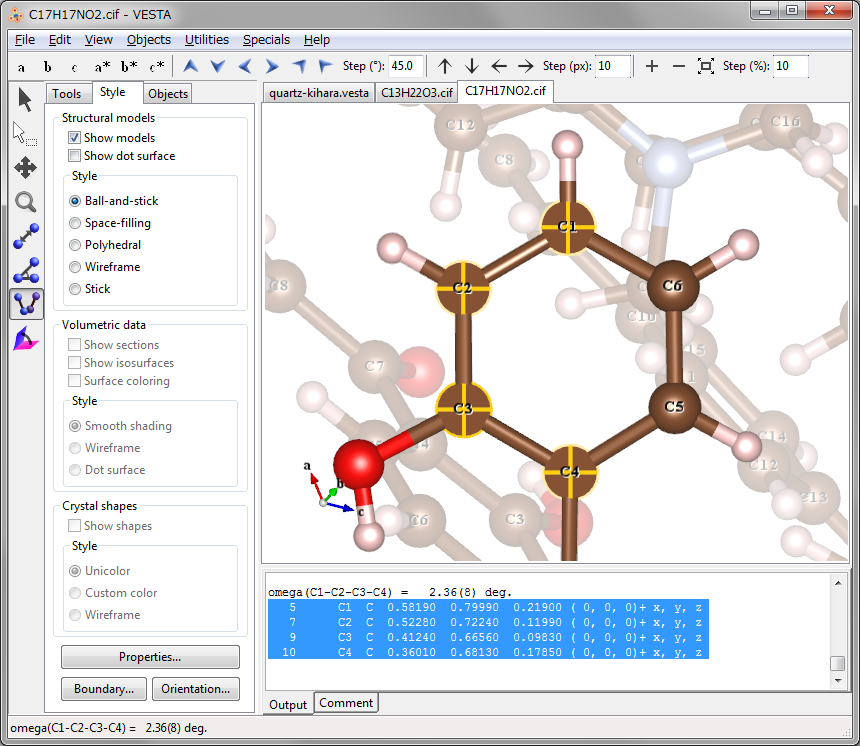
omega(C1-C2-C3-C4) =   2.36(8) deg.
   5      C1  C  0.58190  0.79990  0.21900 ( 0, 0, 0)+ x, y, z
   7      C2  C  0.52280  0.72240  0.11990 ( 0, 0, 0)+ x, y, z
   9      C3  C  0.41240  0.66560  0.09830 ( 0, 0, 0)+ x, y, z
  10      C4  C  0.36010  0.68130  0.17850 ( 0, 0, 0)+ x, y, z
Data in lines No. 2\(-\)5 (selected lines in the Text Area in Fig. 11.2) can be used when imposing nonlinear restraints on the dihedral angle in Rietveld refinement with RIETAN-FP [12].
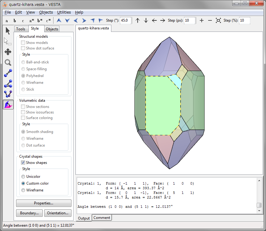
11.8 Interfacial angle
To calculate an interfacial angle, i.e., an angle between two crystal faces, select the eighth button in the Vertical Toolbar. In this mode, only crystal faces can be selected. Selection of a pair of faces A and B gives an angle between their normal vectors (Fig. 11.3).