Chapter 9
ADDITIONAL OBJECTS
9.1 Vectors on Atoms
To attach vectors (arrows) to part of atoms, choose “Edit” menu \(\Rightarrow \) “Vectors…”. These arrows serve to represent magnetic moments or directions of static and dynamic displacements of atoms. At the top of the Vectors dialog box (Fig. 9.1), select a phase to edit. When option “Preview” is checked (default), changes in the dialog box are reflected in the Graphics Area in real time.
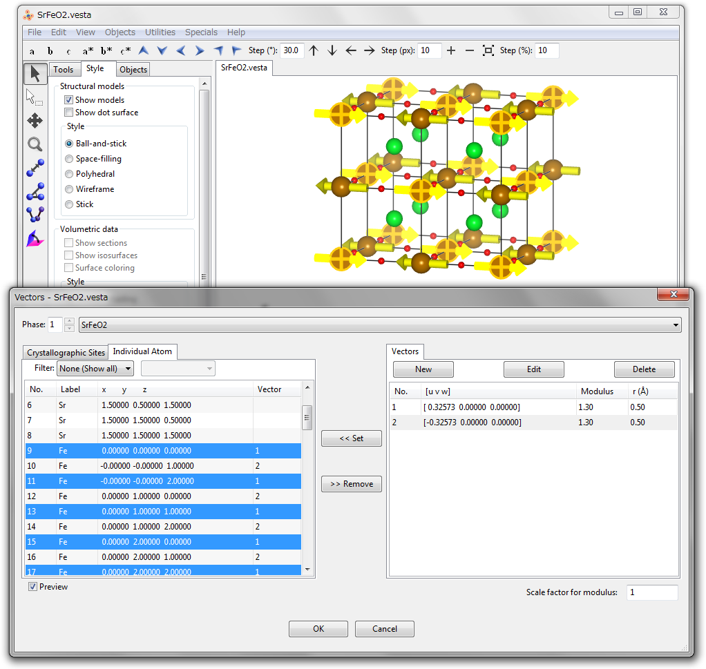
Vectors can be assigned to either crystallographic sites or individual atoms in the Graphic Area. When a vector is attached to a crystallographic site, all of its symmetrically equivalent atoms will bear the same vector, which is properly rotated in accordance with symmetry operations applied to the atoms. When a vector is assigned to each atom, only that atom will have the vector whereas no other symmetrically equivalent atoms will bear the vector. Multiple numbers of vectors can be attached to atoms and sites, and a vector can be attached to more than two atoms and sites. The length of arrows, which are vectors rendered in the Graphics Area, is scaled by moduli of the vectors multiplied by the input value of the {Scale factor for modulus}. For more details about the scaling of vectors, see 9.1.1 and Fig. 9.4.
9.1.1 Creation and editing of a vector
At the right pane of the Vectors dialog box, all the vectors are listed with the following three buttons placed above the list (Fig. 9.1):
| [New]: | Add a new vector. |
| [Edit]: | Edit the selected vector. |
| [Delete]: | Delete the selected vector. |
The [Edit] and [Delete] buttons cannot be clicked unless a vector in the list has been selected.
Click the [New] button to create a new vector. Select a vector in the list of vectors, and click the [Edit] button to edit it. Then, a dialog box appears to edit properties of the selected vector (Fig. 9.2).
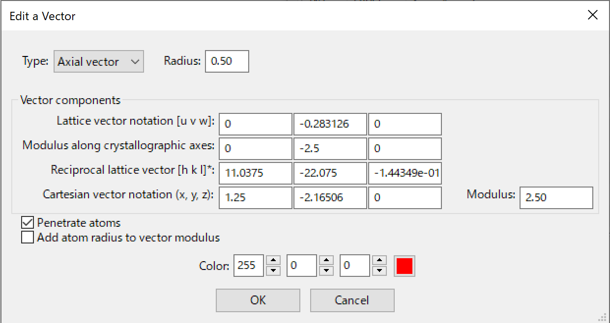
Two types of vectors can be specified: {Axial vector} and {Polar vector}. Because these two differ from each other in the mode of applying symmetry operations, the vector type affects only vectors attached to crystallographic sites. When a vector is attached to individual atoms, no symmetry operation is applied to the vector, with no differences between the two types of the vectors.
Typical examples of axial and polar vectors are magnetic moment, \(\bm {\mu }\), and electrostatic polarization vector, \(\bm {p}\), respectively. The magnetic moment is induced by tiny electrical currents resulting from electrons moving around the nucleus of an atom. The direction of the moment vector is determined by that of the current. For example, counter-clockwise and clockwise currents generate upward and downward moment vectors, respectively. A mirror plane perpendicular to the moment vector does not change the current direction, while a mirror plane parallel to the moment vector inverses the current direction. As a result, magnetic moments are transformed by a mirror plane as Fig. 9.3A illustrates.
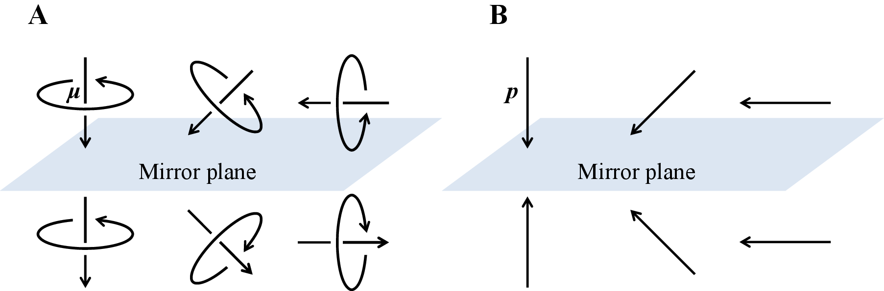
In the case of the electrostatic polarization vector, on the other hand, a mirror plane perpendicular to the moment vector inverses the polarization vector, while a mirror plane parallel to the polarization vector does not change the polarization vector (Fig. 9.3B). To be more specific, \(\bm {p}\) is transformed to \(\bm {p}^\prime \) by a \(3 \times 3\) operator matrix, \(\bm {M}\), as \begin {equation} \bm {p}^\prime = \bm {Mp} \end {equation} while \(\bm {\mu }\) is transformed to \(\bm {\mu }^\prime \) as \begin {equation} \bm {\mu }^\prime = P\bm {M} \bm {\mu }, \end {equation} where \(P\) is the determinant of \(\bm {M}\) and referred to as the “parity” of the operator \(\bm {M}\). Note that the term \(P\bm {M}\) is a scalar-matrix multiplication.
Aside from conventional symmetry operations \(\bm {M}\), there is another important symmetry element for vectors, i.e. time reversal. In view of time reversal, the current direction around an atom is changed, with a result that the direction of \(\bm {\mu }\) is reversed. Let the time reversal be \(T\) (\(=1\) or \(-1\)), then the transformation of \(\bm {\mu }\) is represented by \begin {equation} \bm {\mu }^\prime = TP \bm {M} \bm {\mu }. \end {equation} For the polarization vector, time reversal has no effect at all.
In the Edit a Vector dialog box, three different representations of vector components are shown: {Lattice vector notation (u, v, w)}, {Modulus along crystallographic axes}, and {Cartesian vector notation (x, y, z)}. Editing one representation of the vector components updates the rest of the representations as well as the {Modulus} of the vector. After the {Modulus} has been edited, vector components are linearly scaled.
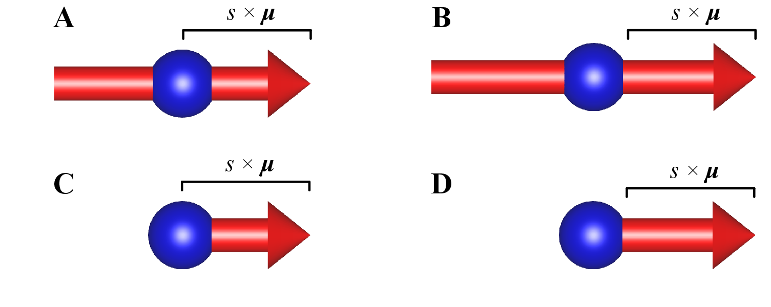
When the “Penetrate atoms” check box is on (default), the length of an arrow (vector drawn in the Graphic Area) is doubled with its center placed at the center of an atom (Figs. 9.4A and 9.4B). When this option is off, one end of an arrow is placed at the center of an atom so that it appears only one side above the atom sphere (Figs. 9.4C and 9.4D).
When option “Add atom radius to the vector modulus” is checked, the length of an arrow appearing above an atom sphere is linearly scaled by the vector modulus, regardless of the radius of the atom sphere (Figs. 9.4B and 9.4D). Even if a vector with a very small modulus is attached to an atom having a very large sphere, the arrow will not be hidden by the atom sphere. If this option is disabled (default behavior), the arrow length including the part hidden by an atom sphere is linearly correlated to the vector modulus(Figs. 9.4A and 9.4C); consequently, a very short arrow may be completely hidden by the atom sphere.
9.1.2 Attachment of vectors to crystallographic sites
To attach a vector to crystallographic sites, select the Crystallographic sites tab at the left pane of the Vectors dialog box. Then, select sites in the left pane, select a vector in the right pane, and click the [\(<<\) Set] button. In a similar manner, select crystallographic sites in the left pane, and click the [\(>>\) Remove] button to detach a vector from the sites.
9.1.3 Attachment of vectors to individual atoms
To attach a vector to individual atoms in the Graphics Area, select the Individual atoms tab at the left pane of the Vectors dialog box. Select atoms from a list in the left pane or by clicking atoms in the Graphics Area. Then, select a vector in the right pane of the Vectors dialog box, and click the [\(<<\) Set] button. In a similar manner, select atoms in the left pane, and click the [\(>>\) Remove] button to detach a vector from the atoms. When atoms in the list in the left pane are selected, the corresponding ones are highlighted in the Graphics Area, and vice versa.
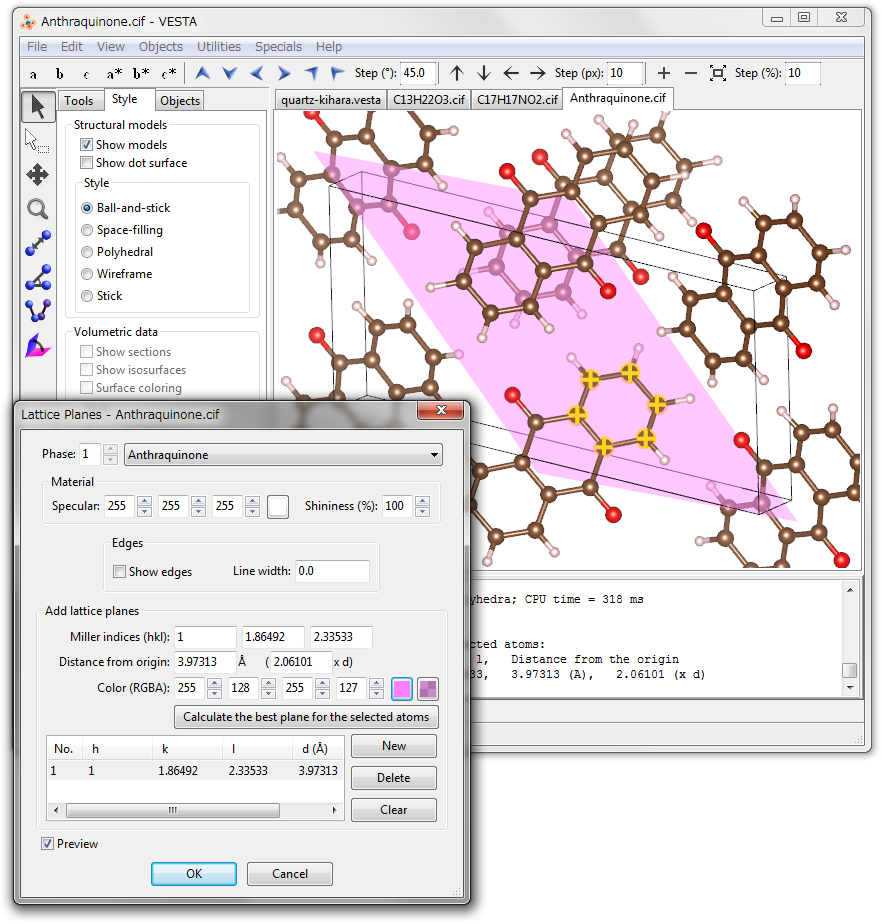
9.2 Lattice Planes
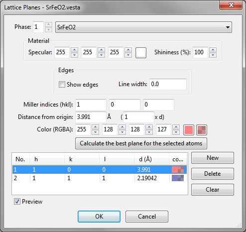
To insert lattice planes in structural models, or to add 2D slices of volumetric data in 3D images, choose “Edit” menu \(\Rightarrow \) “Lattice Planes…”. At the top of the Lattice Planes dialog box (Fig. 9.5), select a phase to edit. A list of lattice planes is shown at the lower half of the dialog box. Some of buttons and text boxes are disabled when no lattice plane is selected in the list. On selection of an item in the list, the text boxes are updated to show data relevant to the selected lattice plane. When option “Preview” is checked (default), changes in the dialog box are reflected in the Graphics Area in real time.
To add a new lattice plane, click the [New] button at first, input Miller indices \(hkl\), and the distance from the origin, (0, 0, 0). The distance may be specified in the unit of either its lattice-plane spacing, \(d\), or Å. The color and opacity of the lattice plane is specified either as four integers ranging from 0 to 255 or from a color selection dialog box, which is opened after clicking the square button on the right side of the text boxes.
To delete a lattice plane, select an item in the list, and then click the [Delete] button or press the \(<\)Delete\(>\) key. Clicking the [Clear] button deletes all the lattice planes in the list.
9.2.1 Appearance of lattice planes
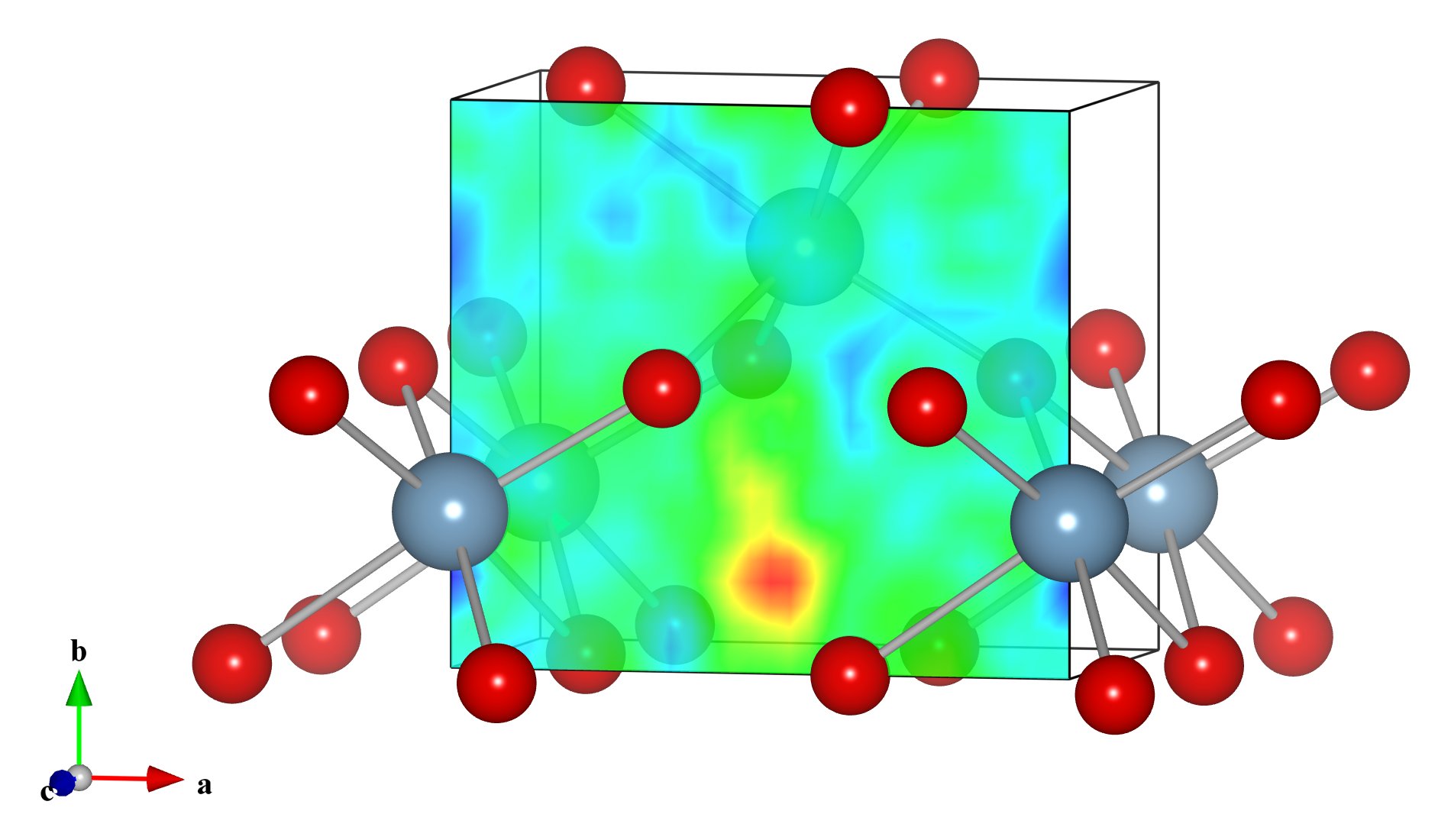
When volumetric data are included in the current data, lattice planes are colored according to volumetric data on the lattice planes. Saturation levels of colors are specified at Sections page in the Properties dialog box (Fig. 9.6; see 12.1.6). When only structural information is included in the current data, lattice planes are drawn with colors specified in this dialog box. To draw lattice planes with specified colors for data having both structural and volumetric information, volumetric data should be deleted at the Edit Data dialog box (see 6.4).
Material settings of lattice planes, i.e. specular color and shininess are input in the Material frame box. Drawing of edges for lattice planes can be controlled in the Edge frame box. These settings are common to all the lattice planes.
9.2.2 Calculate the best plane for selected atoms
To calculate the best plane for a group of atoms (Fig. 9.7), add a new lattice plane at first, select three or more atoms in the Graphics Area, and press [Calculate the best plane for the selected atoms] button.