
Chapter 18
INPUT AND OUTPUT FILES
18.1 Files Used by VESTA
| asfdc |
A file storing parameters related to atomic form factors. |
| element.ini |
A file storing default colors and radii of atoms. |
| spgra.dat |
A file storing information on 230 space groups, e.g., coordinates of equivalent positions compiled in International Tables for Crystallography, volume A [30]. |
| spgro.dat |
A file storing non-conventional symbols of orthorhombic space groups. |
| wyckoff.dat |
A file storing information on wyckoff positions. |
| mspgr.dat |
A file storing information on 1651 magnetic space groups. |
| style.ini |
Default file for styles of the graphic scene. |
| template.ins |
A template file for the standard input of RIETAN-FP [12]. It is used for exporting *.ins and simulating of powder diffraction patterns. |
| VESTA_def.ini |
Default file for various settings of VESTA. |
| $USER_DIR/VESTA.ini\(^{\dagger }\) |
A file for user settings of VESTA. This file is copied from VESTA_def.ini when VESTA is executed for the first time by the user. |
| $USER_DIR/style/default.ini\(^{\dagger }\) |
User settings file for styles of the graphic scene. This file is copied from style.ini when VESTA is executed for the first time by the user. |
\(^{\dagger }\) $USER_DIR is a directory for user settings (see 18.2).
18.2 Directories for User Settings
VESTA loads and saves two files, VESTA.ini and style/default.ini in a directory for user settings to store user settings for the program and for graphics, respectively. A directory, tmp, to store temporary files is also created in the same directory. The location of the settings directory depends on operating systems, and is determined in the following order of priority.
18.2.1 Windows
- When environmental variable VESTA_PREF is defined, the specified directory is used.
- When a directory named VESTA exists in %HOMEPATH%\AppData\Roaming\, it is used. (%HOMEPATH% represents the full path of the user’s home directory, and %HOMEPATH%\AppData\ is a hidden directory.)
- When the user has permission to write in the program directory of VESTA, that directory is used so as not to put the home directory in disorder.
- A directory %HOMEPATH%\AppData\Roaming\VESTA\ is created on the first execution of VESTA to use it.
18.2.2 macOS
- When environmental variable VESTA_PREF is defined, the specified directory is used. To define environmental variables for GUI applications, they must be described in a text file named environment.plist under a hidden directory, ~/.MacOSX. To make it easier to define VESTA_PREF, a utility called set_VESTA_PREF.app is included in the RIETAN-VENUS package1 ; refer to Readme_mac.pdf for details in set_VESTA_PREF.app.
- A directory ~/Library/Application Support/VESTA/ is created on the first execution of VESTA, and it is used. Note that ~/Library is a hidden directory under the home directory (~/).
18.2.3 Linux
- When environmental variable VESTA_PREF is defined, the specified directory is used.
- A hidden directory ~/.VESTA/ is created on the first execution of VESTA to use it.
18.3 File Formats of Volumetric Data
Volumetric data are composed of regular grids in 3D space. A volume element, “voxel,” at each grid point represents a value on the grid point. Voxels are analogous to pixels, which represent 2D image data.
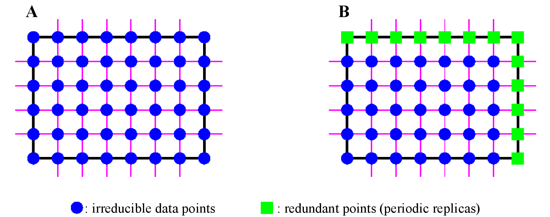
In general, two types of formats are used to record volumetric data in files: general and periodic grids. Figure 18.1 schematically illustrates the general concepts of the two kinds of the formats.
The general grid is a uniform one spanned inside a bounding box for molecules and a unit cell for crystals. For crystal structures, part of data in the general grid are redundant owing to the periodicity of the data. For example, a numerical value at (1, 1, 1) are equal to that at the origin, i.e, (0, 0, 0). Grids where these redundant points have been omitted are called periodic ones.
VESTA distinguishes the grid types automatically from file extensions. For volumetric data with the periodic grid format, VESTA internally generates the general grid by adding redundant data points. On preparation of volumetric data using a self-made script or a program, the user must pay attention to the grid type of a file by himself.
18.4 File Format of *.pgrid and *.ggrid
Both *.pgrid and *.ggrid files have the same format of header data followed by binary data of each voxel. The main difference between the two file formats is that data in *.pgrid are the periodic grid whereas data in *.ggrig are the general grid. Part of the C++ source code to output these files are as follows.
int version[4] = {3, 0, 0, 0}; //The current version number is 3 0 0 0
int gType; // 0: general grid (*.ggrid); 1: periodic grid (*.pgrid).
int fType; // 0: raw data; 1: paired record of index and value of voxel.
int nVal; // 1 or 2; Number of data values for each voxel.
int dim; // Only dimension=3 is currently supported.
int nVox[3]; // Number of voxels along a, b, and c axis.
// Total number of voxels to be recorded in the file.
// nAsym = nVox[0]*nVox[1]*nVox[2] in the case of fType = 1.
int nAsym;
float cell[6]; // Unit cell parameters: a, b, c, alpha, beta, gamma
// Allocate voxel data
float *rho = new float[nVox[0] * nVox[1] * nVox[2]];
// Set values to the above parameters before writing them.
// Write header
fwrite(version, sizeof(int), 4, fptr);
fwrite(title, sizeof(title), 1, fptr);
fwrite(&gType, sizeof(int), 1, fptr);
fwrite(&fType, sizeof(int), 1, fptr);
fwrite(&nVal, sizeof(int), 1, fptr);
fwrite(&dim, sizeof(int), 1, fptr);
fwrite(nVox, sizeof(int), 3, fptr);
fwrite(&nAsym, sizeof(int), 1, fptr);
fwrite(cell, sizeof(float), 6, fptr);
For the raw data type (when fType = 0), binary data of each voxel is output in the following order.
for(int k=0; k<nVox[2]; k++){
for(int j=0; j<nVox[1]; j++){
for(int i=0; i<nVox[0]; i++){
m = k*nVox[0]*nVox[1] + j*nVox[0] + i;
fwrite(&rho[m], sizeof(float), 1, fptr);
}
}
}
}
Note that values of nVox are not the same in the case of fType = 0 (*.ggrid) and fType = 1 (*.pgrid). When saving periodic data in the former format, i.e., as the general grid format, each value of nVox is 1 voxel larger than that of the latter format. The difference is due to the redundant data points at \(x = 1\), \(y = 1\), and \(z = 1\), which are recorded in *.ggrid but not in *.pgrid. For non-periodic data, always use *.ggrid instead of *.pgrid.
When the data is periodic and space group symmetry is higher than -1, the file size can be reduced by only recording data of symmetrically independent voxels. In this case, set the parameter fType = 1 and write a list of symmetry operations before voxel data.
int nPos; // Number of symmetry operations to be written.
// nCen: A flag if the recorded symmetry operations need to be expanded by
// inversion operation.
// 0 for non-centrosymmetric space groups or when all symmetry operations
// are recorded.
// 1 for centrosymmetric and only half of symmetry operations are recorded.
// VESTA and Dysnomia always record full set of symmetry operations and set
// nCen=0 to allow arbitrary origin shift.
int nCen;
// nSub: Number of lattice points.
// nSub>1 in the case of complex lattices such as I, F, A, B, C etc.
// VESTA and Dysnomia always record full set of symmetry operations and set
// nSub=1 to allow arbitrary origin shift.
int nSub;
// A list of lattice points in integer.
// For the P-lattice, or when all symmetry operations are recorded,
// subPos[1][3] = {0, 0, 0};
// subPos[2][3] = {{0, 0, 0},{nVox[0]/2, nVox[1]/2, 0}}; C-lattice
// subPos[2][3] = {{0, 0, 0},{nVox[0]/2, nVox[1]/2, nVox[2]/2}}; I-lattice
// etc.
int subPos[NSUB][3];
// A 4x4 matrix class storing symmetry operation in column-major format.
// The first 3x3 part represent rotation.
// The 4th column represent translation.
// An operator (i,j) in the following code is defined to return a value of
// i-th raw and j-th column in double.
Matrix *symOP;
// A list of indices of voxel positions in asymmetric unit.
int *ijk;
// Set values to the above parameters before writing them.
if(fType = 1){
fwrite(&nPos, sizeof(int), 1, fptr);
fwrite(&nCen, sizeof(int), 1, fptr);
fwrite(&nSub, sizeof(int), 1, fptr);
// Write symmetry operations
// A position X is transformed to X’ by X’ = symOP[i] * X.
for(i=0; i<nPos; i++){
for(j=0; j<3; j++){
for(k=0; k<3; k++){
int a = (int)(symOP[i](k,j));
fwrite(&a, sizeof(int), 1, fptr);
}
}
for(j=0; j<3; j++){
int a = (int)(symOP[i](j,3) * nVox[j]);
fwrite(&a, sizeof(int), 1, fptr);
}
}
for(i=0; i<nSub; i++){
fwrite(subPos[i], sizeof(int), 3, fptr);
}
// Write voxel data in asymmetric unit.
// ijk is 3 indices of position of i_th voxel.
for(i=0; i<nAsym; i++){
m = ijk[i*3+2]*nVox[0]*nVox[1] + ijk[i*3+1]*nVox[0] + ijk[i*3];
fwrite(&m, sizeof(int), 1, fptr);
fwrite(&rho[m], sizeof(float), 1, fptr);
}
}
18.5 Supported File Formats
Input
1. dummy
Structure data
- 1.
- VESTA format (*.vesta)
- 2.
- VICS format (*.vcs)
- 3.
- AMCSD format (*.amc)
- 4.
- ASSE format (*.asse)
- 5.
- Chem3D format (*.cc1)
- 6.
- CIF (*.cif)
- 7.
- CrystalMaker text file (*.cmtx)
- 8.
- CSSR (*.cssr)
- 9.
- CSD/FDAT (*.csd,*.fdt)
- 10.
- DL_POLY (CONFIG, REVCON)
- 11.
- FEFF (feff.inp)
- 12.
- FHI-aims input file(*.in)
- 13.
- Elk FP-LAPW (GEOMETRY.OUT)
- 14.
- GSAS format (*.exp)
- 15.
- ICSD format (*.ics)
- 16.
- ICSD-CRYSTIN (*.cry)
- 17.
- MDL Molfile (*.mol)
- 18.
- MINCRYST (*.min)
- 19.
- MOLDA (*.mld)
- 20.
- Protein Data Bank (*.pdb)
- 21.
- RIETAN-FP input file(*.ins)
- 22.
- RIETAN-FP output file (*.lst)
- 23.
- SHELXL (*.ins, *.res)
- 24.
- STRUCTURE TIDY (*.sto)
- 25.
- USPEX output file (POSCARS)
- 26.
- WIEN2k (*.struct)
- 27.
- XMol XYZ (*.xyz)
- 28.
- SCAT and contrd (*.f01, C04D)
- 29.
- MXDORTO/MXDTRICL
- 30.
- XTL format (*.xtl)
Volumetric data
- 31.
- PRIMA binary format (*.pri)
- 32.
- MEM text format (*.den)
- 33.
- Energy Band (*.eb)
- 34.
- General volumetric-data (text format) (*.?ed)
- 35.
- Periodic volumetric-data (text format) (*.grd)
- 36.
- General volumetric-data (binary format) (*.ggrid)
- 37.
- Periodic volumetric-data (binary format) (*.pgrid)
- 38.
- Compressed volumetric-data (*.m3d)
- 39.
- SCAT volumetric-data (*.sca, *.scat)
- 40.
- WIEN2k (*.rho)
- 41.
- WinGX 3D Fourier map (*.fou)
- 42.
- X-PLOR/CNX (*.xplor)
Structure and volumetric data
- 43.
- CASTEP (*.cell, *.charg_frm)
- 44.
- GAMESS (*.inp,*.mmp)
- 45.
- Gaussian (*.cube, *.cub)
- 46.
- VASP (*.vasp, CHGCAR, etc.)
- 47.
- XCrySDen XSF format (*.xsf)
Output
Structure data
- 1.
- VESTA format (*.vesta)
- 2.
- Chem3D format (*.cc1)
- 3.
- CIF (*.cif)
- 4.
- DL_POLY CONFIG format (*.config)
- 5.
- Protein Data Bank (*.pdb)
- 6.
- RIETAN-FP (*.ins)
- 7.
- SHELXL (*.ins)
- 8.
- XMol XYZ (*.xyz)
- 9.
- P1 structure (*.p1)
- 10.
- Fractoinal coordinates (*.xtl)
- 11.
- MADEL input files (*.pme)
- 12.
- TRRUCTURE TIDY (*.stin)
Volumetric data
- 13.
- PRIMA binary format (*.pri)
- 14.
- General volumetric-data (text format) (*.3ed)
- 15.
- Periodic volumetric-data (text format) (*.grd)
- 16.
- General volumetric-data (binary format) (*.ggrid)
- 17.
- Periodic volumetric-data (binary format) (*.pgrid)
- 18.
- Compressed volumetric-data (*.m3d)
- 19.
- X-PLOR/CNX (*.xplor)
Structure and volumetric data
Geometry data
- 22.
- STL file (*.stl)
- 23.
- VRML file (*.wrl)
Graphic image
Raster graphics
- 1.
- BMP (*.bmp)
- 2.
- EPS (*.eps)
- 3.
- JPEG (*.jpg)
- 4.
- JPEG2000 (*.jp2)
- 5.
- PNG (*.png)
- 6.
- PPM (*.ppm)
- 7.
- RAW (*.raw)
- 8.
- RGB (*.rgb)
- 9.
- TGA (*.tga)
- 10.
- TIFF (*.tif)
Vector graphics
18.5.1 Input
Structural data
- 1.
- VESTA format (*.vesta)
Text files containing the entire structure data and graphic settings. File *.vesta saved by VESTA may contain relative paths to volumetric data files and a crystal-data file that are automatically read in when *.vesta is reopened. If any one of keywords, IMPORT_STRUCTURE, IMPORT_ORFFE, IMPORT_DENSITY, and IMPORT_TEXTURE, is included in *.vesta and followed by lines specifying relative paths to data files, these data files are also input by VESTA when *.vesta are opened.
After Rietveld analysis with RIETAN-FP [12], lattice and structure parameters in *.vesta are automatically updated provided that *.vesta and *.ins share the same folder.
- 2.
- VICS format (*.vcs)
http://fujioizumi.verse.jp/visualization/VENUS.htmlVICS, which is the predecessor of the structure-drawing part of VESTA, is now obsolete. Nevertheless, this format is still supported in VESTA to maintain compatibility.
- 3.
- American Mineralogist Crystal Structure Database [99] (*.amc)
http://rruff.geo.arizona.edu/AMS/amcsd.php
In part of AMCSD text files, extra characters are attached to space group names, and non-standard space-group symbols are used. Some of such non-standard space-group settings may not be read in correctly. In such a case, modify the space-group symbol appropriately and then change the setting number in the Unit cell tab of the Edit Data dialog box if necessary. Sometimes, you have to convert fractional coordinates by yourself if a non-standard setting that is not described in International Tables for Crystallography, volume A [30] is adopted.
- 4.
- asse (*.asse)
http://www.nims.go.jp/cmsc/staff/arai/asse/ - 5.
- Chem3D (*.cc1)
http://openbabel.org/docs/2.3.1/FileFormats/3D_viewer_Formats.html - 6.
- Crystallographic Information File (CIF; *.cif) [100]
http://www.iucr.org/resources/cif/
CIF has a variety of formats for crystal data. You can get detailed information about CIF from the above Web site. For example, CIF files may contain Cartesian coordinates, but VESTA cannot input them. Note that VESTA does not support all the formats allowed in the CIF format. For example, Cartesian coordinates included in CIFs cannot be input with VESTA; only fractional coordinates should be given in CIFs. For readable formats, refer to example files of *.cif in VENUS/examples/VICS/CIF.
In the case of *.cif containing multiphase data, all the data are input in the same tab and overlapped with each other. To visualize only one phase in such a case, select “Edit” menu \(\Rightarrow \) “Edit Data” \(\Rightarrow \) “Phase…”. Select an unnecessary phase in the list, and press [Delete] button.
The CIF specification presents multiple ways of inputting entries for space-group symmetry. VESTA searches the entries in the following order:
_symmetry_equiv_pos_as_xyz
_symmetry_space_group_number
_symmetry_space_group_name_H-M
If one of the above entries are given in *.cif, VESTA recognizes space-group symmetry. For example, CIFs created by SHELX-97 [97] through WinGX [101] contain neither space-group number nor space-group symbol but have a list of symmetry operations.
If none of the above entries are correctly given, the space group is regarded as \(P1\). In this case, set the space group in the Unit cell tab of the Edit Data dialog box after opening such a file, or modify a line relevant to the space group in the CIF in the following manner:
_symmetry_space_group_number 12
or
_symmetry_space_group_name_H-M ’P 21/n’
- 7.
- CrystalMaker text file (*.cmt, *.cmtx)
http://www.crystalmaker.comCrystalMaker is a commercial program for building, displaying, and manipulating all kinds of crystal and molecular structures.
- 8.
- Crystal Structure Search and Retrieval (CSSR; *.cssr)
http://www.maciejharanczyk.info/Zeopp/input.htmlIn a file with the CSSR format, a setting numbers may be given after ‘OPT =’. Unfortunately, we have no information about setting numbers in this format. Then, please change it in the Unit cell tab of the Edit Data dialog box if necessary.
- 9.
- Cambridge Structural Database [102] (CSD/FDAT; *.csd, *.fdt))
http://www.ccdc.cam.ac.uk/Solutions/CSDSystem/Pages/CSD.aspx - 10.
- DL_POLY [103] format (CONFIG, REVCON, *.config)
https://www.scd.stfc.ac.uk/Pages/DL_POLY.aspx - 11.
- FEFF input file (feff.inp)
http://www.feffproject.org/
FEFF [104, 105] is an automated program for ab initio multiple-scattering calculations of X-ray Absorption Fine Structure (XAFS) and X-ray Absorption Near-Edge Structure (XANES) spectra for clusters of atoms. The names of input files for FEFF must be either feff.inp or FEFF.INP.
- 12.
- FHI-aims input file (*.in)
https://aimsclub.fhi-berlin.mpg.de/FHI-aims is an accurate all-electron, full-potential electronic structure code package for computational materials science.
- 13.
- Output file of the Elk FP-LAPW Code (GEOMETRY.OUT)
http://elk.sourceforge.net/Elk is an all-electron full-potential linearised augmented-planewave (FP-LAPW) code for determining the properties of crystalline solids.
- 14.
- GSAS [18] format (*.EXP)
http://www.ncnr.nist.gov/xtal/software/gsas.html - 15.
- Inorganic Crystal Structure Database [87] (ICSD; *.ics)
http://www2.fiz-karlsruhe.de/icsd_home.html
Two retrieval programs, RETRIEVE for MS-DOS and FindIt for Windows, of ICSD output text files with quite different formats. VESTA is capable of reading in both types of the crystal data files.
In these *.ics files, extra characters are sometimes attached to space group names, e.g., ’P 42/n m c S’, which should be ’P 42/n m c’ (P\(4_2\)/nmc). In addition, full Hermann-Mauguin space-group symbols are sometimes given in ICSD text files. In such a case, an error message appears in both the Text Area and a message box. Read it carefully to proceed to a next operation. When you encounter this type of an error, it is strongly recommended to output a CIF instead of *.ics.
- 16.
- ICSD-CRYSTIN: (*.cry)
- 17.
- MDL Molfile (*.mol)
http://en.wikipedia.org/wiki/Chemical_table_file - 18.
- MINCRYST (Crystallographic Database for Minerals; *.min)
http://database.iem.ac.ru/mincryst/
In part of MINCRYST text files, extra characters are attached to space group names, and non-standard space-group symbols are used. In such a case, an error message appears in the Text Area. Such space group names need to be appropriately changed. Change the setting number in the Unit cell tab of the Edit Data dialog box if necessary.
- 19.
- MOLDA [106] (*.mld)
http://www3.u-toyama.ac.jp/kihara/cc/mld/readme.htmlThe Web site of MOLDA has been closed because the author, Hiroshi Yoshida passed away in 2005. Then, the MODRAST/MOLDA format for *.mld is briefly explaned here. This format consists of the following lines:
- (a)
- Line No. 1: A comment about the compound, e.g., its name
- (b)
- Line No. 2: Number of atoms, \(n_{\mathrm {a}}\), in the compound
- (c)
- Lines No. \(3-(3+n_{\mathrm {a}})\): Cartesian coordinates (\(x\), \(y\), and \(z\)) and an atomic number
- (d)
- Line No. \((4+n_{\mathrm {a}})\): Number of bonds, \(n_{\mathrm {b}}\), in the compound
- (e)
- Lines No. \((5+n_{\mathrm {a}})-(5+n_{\mathrm {a}}+n_{\mathrm {b}})\): A pair of atom numbers
For example, in the case of ethylene, where \(n_{\mathrm {a}} = 6\) and \(n_{\mathrm {b}} = 5\), the following lines are required:
"Ethylene (CH2=CH2)"
6
.66958, 0, 0, 6
1.23873, -.94397, 0, 1
1.23873, .94397, 0, 1
-.66958, 0, 0, 6
-1.23873, -.94397, 0, 1
-1.23873, .94397, 0, 1
5
1, 4
1, 2
1, 3
4, 5
4, 6
- 20.
- Protein Data Bank (PDB; *.pdb) [107]
http://www.wwpdb.org/
PDB has a variety of formats for crystal data. You can get detailed information on PDB in a Web page http://www.wwpdb.org/docs.html. Note that VESTA does not support all the formats allowed in these two formats. For readable formats, refer to *.pdb in VENUS/examples/VICS/PDB.
- 21.
- Input file of RIETAN-FP/2000 [12, 108] (*.ins)
http://fujioizumi.verse.jp/download/download_Eng.htmlVESTA cannot input *.ins for versions of RIETAN (e.g., RIETAN-94) earlier than RIETAN-2000. In the case of *.ins containing multiphase data, only the crystal data of the first phase are input.
In *.ins, the volume name of International Tables should be not ’I’ but ’A’ in accordance with a specification in RIETAN-FP. For example, ’A-230-2’ is input for the second setting of space group \(Fd\bar {3}m\). The input of ’I-230-2’ causes an error. Lattice parameters must be given within one line in the following way:
CELLQ 9.36884 9.36884 6.88371 90.0 90.0 120.0 0.0 1010000 - 22.
- Output file of RIETAN-FP [12] (*.lst)
http://fujioizumi.verse.jp/download/download_Eng.htmlBeware lest *.lst output by RIETAN-2000 [108] is input.
- 23.
- SHELXL [97] (*.ins)
- 24.
- Output file of STRUCTURE TIDY (*.sto)
- 25.
- Structure data files output by USPEX (gatheredPOSCARS, BESTgatheredPOSCARS) [109, 110]
http://han.ess.sunysb.edu/˜USPEX/ - 26.
- WIEN2k [41] (*.struct)[109, 110]
http://www.wien2k.at/ - 27.
- XMol XYZ (*.xyz)
http://en.wikipedia.org/wiki/XYZ_file_format
http://openbabel.org/docs/2.3.1/FileFormats/XYZ_cartesian_coordinates_format.htmlXMol developed at the Minnesota Supercomputer Center is a utility for creating and viewing graphic images of molecules.
- 28.
- F01 for SCAT [58, 111] and C04D for contrd
http://www.dvxa.org/
VESTA need to read in c04d, which is an input file of contrd, in addition to f01 if a structural model is to be overlap with volumetric data. For this purpose, the dimensions of a boundary box (an area where volumetric data are output to text files) in c04d are required. For details in contrd, refer to Readme_contrd.txt in the VENUS package [15, 16]. Of course, c04d and f01 should be placed in the same folder. If c04d has not been input by VESTA, atomic coordinates are treated in the Cartesian coordinate system, as is the case for *.xyz files. In this case, volumetric data, *.scat and *.sca, cannot be overlapped with the structural model.
All the atoms recorded in f01 must be included within the above boundary box. Otherwise, atomic coordinates are normalized within the boundary box by assuming periodicity, which leads to the appearance of incorrect structures in the Graphics Area.
The assistance environment for the DV-X\(\alpha \) method2 using Hidemaru Editor is very convenient when carrying out a series of electronic-state calculations.
The Web site of Genta Sakane of Okayama University of Science:
http://www.chem.ous.ac.jp/˜gsakane/
is very useful for those who like to visualize physical quantities calculated with contrd. “Introduction to the assistance environment for the DV-X\(\alpha \) method3 ” distributed there is a detailed Japanese document suitable for beginners in the DV-X\(\alpha \) method as well as VESTA. - 29.
- MXDORTO/MXDTRICL [112, 113] (FILE06.DAT, FILE07.DAT)
http://kats-labo.jimdo.com/mxdorto-mxdtricl/MXDORTO and MXDTRICL are Fortran programs for molecular dynamics simulation.
- 30.
- XTL format (*.xtl)
Text files used in Cerius2 (Accelrys, Inc.4 ). GULP [114] and GSAS [18] are capable of outputting crystal data with this format.
Volumetric data
- 31.
- MEM densities in binary format (*.pri, *.prim)
http://fujioizumi.verse.jp/visualization/VENUS.html
http://jp-minerals.org/dysnomia/en/
Binary files of 3D electron and nuclear densities output by PRIMA [5] or Dysnomia [7, 8] and those of Patterson functions output by ALBA [17]. The unit of electron densities (strictly speaking, number densities of electrons) recorded in these files is Å\(^{-3}\), and that of nuclear densities is fmÅ\(^{-3}\).
- 32.
- MEM densities in text format (*.den)
Text files of 3D electron and nuclear densities output by PRIMA, Dysnomia, MEED [115], MEND [116], and ENIGMA [117]. The unit of electron densities recorded in these files is Å\(^{-3}\) while that of nuclear densities is fmÅ\(^{-3}\).
- 33.
- Energy Band (*.eb)
Text files having practically the same format with *.rho. Files *.eb are used to visualize Fermi surfaces from results obtained with programs for band-structure calculations, e.g., WIEN2k [41]. As a matter of convenience, a constant is added to all the energy eigenvalues in *.eb so as to make them greater or equal to zero. Therefore, the isosurface level has to be set with this padding in mind.
Masao Arai of NIMS provides us with detailed information about *.eb in his Web site:
http://www.nims.go.jp/cmsc/staff/arai/ - 34.
- General volumetric-data (text format) (*.?ed)
A file with the general volumetric-data format stores one of the following physical quantities converted from electron densities according to procedures proposed by Tsirelson [48] (see 14.15):
\(\nabla ^2 \rho (\bm {r})\): \(g(\bm {r})\): \(\nu (\bm {r})\): \(h_{\mathrm {e}}(\bm {r})\): with the format (common to all the files with the extension of ?ed):
Title: Title up to 80 characters.
\(a\), \(b\), \(c\), \(\alpha \), \(\beta \), \(\gamma \): Lattice parameters with at least one space between two parameters (free format).
N1+1, N2+1, N3+1: Numbers of voxels along the \(a\), \(b\), and \(c\) axes, respectively, with at least one space between two integers (free format).
followed by elements of a three-dimensional array, D
(((D(I1, I2, I3), I3 = 1, N3+1), I2 = 1, N2+1), I1 = 1, N1+1)
with any number of data in each line and at least one space between two real data (free format). Note that voxels at N1+1, N2+1, and N3+1 lie on \(x=1\), \(y=1\), and \(z=1\), respectively. A top part of an example of *.ted is given below:
TiO2 (rutile)
   4.59393    4.59393    2.95886   90.00000   90.00000   90.00000
   65    65    65
-3.700291E+004 -3.355551E+004 -2.515189E+004 -1.581991E+004 -8.551052E+003 -4.096268E+003
-1.802126E+003 -7.564262E+002 -3.147750E+002 -1.347187E+002 -6.129182E+001 -3.045389E+001
-1.683229E+001 -1.043066E+001 -7.226008E+000 -5.529954E+000 -4.588889E+000 -4.036150E+000
-3.669965E+000 -3.365605E+000 -3.043458E+000 -2.664371E+000 -2.229370E+000 -1.771544E+000
-1.337361E+000 -9.658093E-001 -6.762105E-001 -4.680259E-001 -3.280885E-001 -2.393913E-001
.....
VESTA allows you to save a file, *.?ed, with the general volumetric-data format. Accordingly, VESTA serves as a converter from a binary file to a text one.
- 35.
- Periodic volumetric-data (text format) (*.grd)
http://www.ncnr.nist.gov/xtal/software/gsas.html
Text files for 3D Fourier maps output by GSAS [18]. A program, 3DBVSMAPPER [118], for automatically generating bond-valence sum images is also capable of outputting files with this format. To create *.grd files that can be input by VESTA, select option “C – Select section (X, Y, or Z) selection” in Fourier calculation setup and then enter “X” for prompt “Enter section desired (X,Y,Z - choose Z for DSN6 maps).”
The file format is essentially the same as the general volumetric-data format, except that the three-dimensional data array, D, are output in the following range:
(((D(I1, I2, I3), I3 = 1, N3), I2 = 1, N2), I1 = 1, N1)
VESTA also allows you to export volumetric data in this format.
- 36.
- General volumetric-data (binary format) (*.ggrid)
- 37.
- Periodic volumetric-data (binary format) (*.pgrid)
- 38.
- Compressed volumetric-data format (*.m3d)
- 39.
- SCAT volumetric-data files (*.sca, *.scat)
http://www.dvxa.org/Electron densities, electrostatic potentials, and wave functions calculated with contrd from files F09 and F39 output by SCAT [58, 111]. Text files (CHG3D.SCA, POT3D.SCA, WXXX-3D.SCA, WXXXU-3D.SCA, and WXXXU-3D.SCA) created with a batch file named contrd.bat can directly be input by VESTA, where XXX denotes an integer assigned to a wave function. To learn details in *.SCA, refer to Readme_contrd.txt distributed as a part of package [15, 16]. Three-dimensional numerical data recorded in *.SCA or *.SCAT are drawn without any conversion.
Units for electron densities, electrostatic potentials, and wave functions are, respectively, bohr\(^{-3}\), Ry (rydberg), and bohr\(^{-3/2}\), where bohr is the atomic unit for length, i.e., 1 bohr = \(a_0\) = 5.29177211 \(\times 10^{-11}\) m = 0.529177211 Å (\(a_0\): Bohr radius), and 1 Ry = \(E_{\mathrm {h}}\)/2 = 2.179 871 9 \(\times 10^{-18}\) J (\(E_h\): hartree).
Refer to No. 23 in 18.5.1 for the assistance environment for the DV-X\(\alpha \) method and its detailed document written in Japanese.
- 40.
- WIEN2k (*.rho)
http://www.wien2k.at/ (WIEN2k)
http://www.nims.go.jp/cmsc/staff/arai/wien/venus.html (wien2venus.py)
A script, wien2venus.py, coded in Python5 by Masao Arai of NIMS makes it possible to export electron densities calculated with WIEN2k [41] to a text file, *.rho, which is in turn visualized by VESTA. The unit of electron densities stored in this file is bohr\(^{-3}\).
- 41.
- WinGX 3D Fourier map (*.fou)
http://www.chem.gla.ac.uk/˜louis/software/wingx/
Text files of 3D Fourier Maps output by WinGX [101]. To create *.fou that can be input with VESTA, open “FOURIER MAP Control Panel” of WinGX from Maps menu \(\rightarrow \) FOURIER MAP \(\rightarrow \) Slant plane. Select “3D Fouier (Beevers-Lipson)” and “Write MarchingCubes File” options and set “Projection” at Z axis. The minimum and maximum of “Summation limits” should be set at 0 and 1 for all of X, Y, and Z axes. A resolution for each axis should be carefully set in view of the following matter.
In this format, data points along each axis are not uniformly distributed but just placed at intervals of given resolutions. When length of an axis is \(L\) and resolution is set at \(d\), the number of data points, nVox, is set at the integer part of \(L/d + 1\). The output files have a general grid format with nearly correct periodicity only if \(L / d\) is close to an integer. It is recommended that special positions lie exactly on data grid. For example, if mirror planes lie at \(x=1/4\) and \(x=3/4\), \(L / d\) should be multiples of 4.
- 42.
- X-PLOR/CNX (*.xplor)
http://en.wikipedia.org/wiki/X-PLOR (CNX)
http://superflip.fzu.cz/ (Superflip)
Superflip [119] is a computer program for ab initio structure solution of crystal structures by the charge-flipping method [120, 121, 122]. Superflip outputs electron densities in the unit cell in file *.x-plor with the X-PLOR format [123], which can be directly visualized by VESTA.
Structural and volumetric data
- 43.
- CASTEP [124, 125] (*.cell, *.charg_frm)
http://www.castep.org/
File *.cell contains crystal-structure data while file *.charg_frm stores electron densities in the unit of Å\(^{-3}\). Only a structural model is visualized when *.cell is opened by VESTA. On the other hand, both a structural model and electron-density distribution are displayed when opening *.charg_frm. Because no unit-cell dimensions are recorded in *.charg_frm, it must be accompanied by *.cell.
- 44.
- GAMESS [126] input and volumetric data files output by MacMolPlt [127]
http://www.msg.ameslab.gov/GAMESS/GAMESS.html (GAMESS)
https://brettbode.github.io/wxmacmolplt/ (MacMolPlt)
A GAMESS input file, *.inp, can readily be obtained from a GAMESS log file, *.log, with MacMolPlt. At first, examine the unit of final Cartesian coordinates of atoms after convergence in this file using a text editor. Then, run MacMolPlt to open *.log. In the Windows menu, select ‘Coordinates’ through the name of *.log and check whether the unit of Cartesian coordinates is Å or bohr (au). The unit should be Å, as is usual with VESTA. If the unit is Bohr, select ‘Convert to Angstroms’ under the Molecule menu. Then, select ‘Input Builder’ through the name of *.log in the Windows menu and click [Write File] to create *.inp storing atomic symbols and Cartesian coordinates.
Next, a volumetric data file, *.mmp, in which the origin of the 3D grid is recorded, has to be output. In the Windows menu, select ‘Surfaces’ through the name of *.log. Specify an item from ‘3D Orbital’, ‘3D Total Electron Density’, and ‘3D Molecular Electrostatic Potential’. In the dialog box that appears subsequently, change the number of grid points and grid size appropriately, select an orbital (in the case of ‘3D Orbital’), and click [Update]. An isosurface plus a ball-and-stick model appear in the *.log window. The number of grid points, origin, and grid increment are displayed by clicking [Parameters...]. Then, click [Export...]. Specify the name and location of *.mmp with the same basename as *.inp. Note that *.inp and *.mmp must share the same folder.
- 45.
- Gaussian Cube format (*.cube, *.cub)
http://www.gaussian.com/
Text files storing electron densities, spin densities, electrostatic potentials, wave functions, and so forth calculated with Gaussian [128, 129] with a keyword of ‘Cube’.6 .
Cube files can also be created by Firefly (previously known as PC GAMESS).7
- 46.
- VASP (*.vasp, CHG, CHGCAR, PARCHG, LOCPOT, ELFCAR, POSCAR, CONTCAR)
http://www.vasp.at/
http://www.materialsdesign.com/medea (commercial software MedeA including VASP as its component)
All the above files are text files storing crystal-structure and volumetric data output by VASP [130, 131].
CHG stores lattice vectors, atomic coordinates, and total charge densities multiplied by the unit-cell volume, \(V\). PAW one-center occupancies are added to them in CHGCAR. Though both CHG and CHGCAR provide us with the same information on the valence charges, the file size of CHG is smaller than that of CHGCAR owing to the lower accuracy of the numerical data. PARCHG has the same format as CHG has, storing partial charge densities of a particular k-point and/or band. When these files are read in to visualize isosurfaces and sections, data values are divided by \(V\) in the unit of bohr\(^3\). The unit of charge densities input by VESTA is, therefore, bohr\(^{-3}\).
LOCPOT contains lattice vectors, atomic coordinates, and Coulomb potentials (unit: eV), i.e., total potentials without exchange-correlation contributions (unless the line of LEXCHG=\(-\)1 is commented out in main.F). ELFCAR, which has the same format as CHG has, stores dimensionless electron localization functions (ELF). POSCAR and CONTCAR include lattice vectors, atomic coordinates, and optionally starting velocities and predictor-corrector coordinates for molecular-dynamics calculation. POSCAR and CONTCAR, respectively, correspond to the initial structure and the final one output by VASP at the end of a job; CONTCAR can be used to continue the job.
Owing to the absence of symbols of elements or atomic numbers in these files, they must accompany another file, OUTCAR, to display structural models. OUTCAR may be renamed *.out having the same basename as *.vasp has. Only lines following ‘POTCAR:’ at the top part of OUTCAR are required to obtain symbols of elements.
When files are read in for surface coloring, no data values are scaled unless the file name is CHGCAR or PARCHG.
- 47.
- XCrySDen XSF format (*.xsf)
http://www.xcrysden.org/ (XCrySDen)
http://www.abinit.org/ (ABINIT)
http://www.abinit.org/documentation/helpfiles/for-v6.4/users/cut3d_help.html (Cut3D)
http://www.quantum-espresso.org/ (Quantum ESPRESSO)
The ABINIT package [132] for the ab initio computation of material properties has a feature to output binary files storing electron densities, electrostatic potentials, and wave functions. They can be converted into text files, *.xsf, having the XSF format of XCrySDen [133, 134] using a converter named Cut3D. The unit of electron densities is bohr\(^{-3}\). Cut3D supports data Type 13 (XCrySDen/VENUS wavefunction real data), whereby wave functions can be directly output in *.xsf.
Quantum ESPRESSO [135] for quantum simulations of materials has also a feature to output files with the XSF format.
Detailed information about the XSF format can be obtained from
http://www.xcrysden.org/doc/XSF.html
In general, *.xsf consists of some sections that begins with keywords. VESTA reads in volumetric data from a BEGIN_BLOCK_DATAGRID section. To make it possible to overlap isosurfaces with a structural model, *.xsf should also contain (1) PRIMEVEC and PRIMCOORD sections or (2) CONVVEC and CONVCOORD sections. Furthermore, lattice vectors in the PRIMVEC or CONVVEC section must agree with spanning vectors in the BEGIN_DATAGRID section. The unit of primitive lattice vectors (PRIMVEC) and Cartesian coordinates is Å in the XSF format.
18.5.2 Output Files
Structure data
- 1.
- Original format of VESTA (*.vesta)
The entire information about data displayed currently are saved in a text file, *.vesta, with the VESTA format. Files with the VESTA format contains all the structural data and graphic settings whereas volumetric data are not directly recorded in *.vesta but imported from external files. Directories and names of files storing volumetric data are recorded in *.vesta as relative paths to the volumetric-data files from the directory of *.vesta, which makes it possible to save the entire information about the current data in a small file without duplicating huge volumetric data.
Structural data can be optionally imported from an external file in the same manner. To prevent the structural data from being recorded directly in *.vesta, import structural data using the Import Data dialog box with option “Link” (see 6.3.6). A name of file *.ffe output by ORFFE [45] is also recorded in *.vesta so that geometrical parameters recorded in *.ffe are automatically listed in the Geometrical Parameters dialog box after reopening *.vesta (see 14.2). After Rietveld analysis with RIETAN-FP [12], lattice and structure parameters in *.vesta are automatically updated provided that *.vesta and a standard input file, *.ins, share the same folder.
- 2.
- Chem3D (*.cc1)
http://openbabel.org/docs/2.3.1/FileFormats/3D_viewer_Formats.html - 3.
- Crystallographic Information File (CIF; *.cif)
http://www.iucr.org/resources/cif/ - 4.
- DL_POLY CONFIG format (*.config)
https://www.scd.stfc.ac.uk/Pages/DL_POLY.aspx - 5.
- Protein Data Bank (PDB; *.pdb)
http://www.wwpdb.org/ - 6.
- SHELXL [97] (*.ins)
- 7.
- User input file of RIETAN-FP/2000 (*.ins)
http://fujioizumi.verse.jp/download/download_Eng.htmlThe feature of outputting *.ins enables us to read in crystal data files of various formats with VESTA, simulate powder diffraction patterns, and carry out subsequent Rietveld refinements with RIETAN-FP [12]. Note that standard input files of RIETAN-2000 [108] and RIETAN-FP are incompatible with each other. VESTA uses a template file to export input files of RIETAN-FP/2000, and the default template file, template.ins, has the RIETAN-FP format. If a standard input file with the RIETAN-2000 format is desired, change the template file to a file with the RIETAN-2000 format in the Preferences dialog box (see 16).
In Rietveld refinement or simulations of powder diffraction patterns with RIETAN-FP, the following standard lattice settings of STRUCTURE TIDY [85, 46] embedded in RIETAN-FP should be selected:
- Monoclinic system: \(b\)-axis unique setting (\(\beta \ne 90\)°),
- Trigonal system: hexagonal lattice (\(a = b \ne c\) and \(\gamma = 120\)°),
- Centrosymmetric space groups: an inversion center at the origin (origin choice 2 in Ref. [30]).
Unless these three standard settings are adopted, LAZY PULVERIX [86], which is also incorporated in RIETAN-FP, fails in generating correct diffraction indices \(hkl\) and their multiplicities. Accordingly, VESTA automatically transforms the lattice setting of a crystal structure to the standard one when exporting *.ins with the RIETAN-FP/2000 [108, 12] format.
It should be pointed out that fractional coordinates in part of crystal data recorded in databases have too small significant digits, e.g., 0.3333 instead of 0.333333. In such a case, please increase the significant digit to 6 or 7 before outputting *.ins.
- 8.
- XMol XYZ (*.xyz)
http://en.wikipedia.org/wiki/XYZ_file_format
http://openbabel.org/docs/2.3.1/FileFormats/XYZ_cartesian_coordinates_format.html - 9.
- \(P1\) structure (*.p1)
Simple text files storing lattice parameters and atomic positions of all the atoms in the unit cell. Atomic positions are written in fractional coordinates, and the space group of the crystal is converted into \(P1\) (triclinic, No. 1). This format is useful when preparing initial atomic configurations in computational simulations.
- 10.
- Fractional coordinates (*.xtl)
Simple text files with the xtl file format storing atomic positions of all the atoms currently displayed in the Graphics Area. Atomic positions are written in fractional coordinates. The space group of the crystal is treated as \(P1\) (triclinic, No. 1) for convenience.
- 11.
- MADEL input files (*.pme)
Although MADEL can be executed from VESTA (see 14.5), input files of MADEL, *.pme, should be manually edited to calculate electrostatic site potentials of interstitial (vacant) sites, whose fractional coordinates have to be input in FORMAT(3F9.6) at the tail of *.pme. The use of the RIETAN-FP–VENUS integrated assistance environment included in the distribution file of the RIETAN-FP system is highly recommended to edit *.pme and run MADEL to input it on Hidemaru Editor.8 For details in the above assistance environment, read Readme_macros.txt contained in the distribution file.
When exporting files with this format, you are prompted to input two parameters, RADIUS and REGION (see 14.5). Refer to the user’s manual of MADEL for details in these parameters to be input in *.pme.
- 12.
- Input files of STRUCTURE TIDY (*.sto)
Volumetric data
- 13.
- PRIMA binary format (*.pri)
- 14.
- General volumetric-data format (*.3ed)
- 15.
- Periodic volumetric-data format (*.grd)
- 16.
- General volumetric-data format (binary) (*.ggrid)
The general volumetric-data format is the most recommended file format when exporting volumetric data. It is lossless, and yet files with this format have sizes much smaller than those for text formats or even some other binary formats. In the case of periodic volumetric data, *.pgrid described below is preferred because of better compression efficiency. - 17.
- Periodic volumetric-data (binary format) (*.pgrid)
This file format is similar to *.ggrid format but assumes the periodicity of grids to minimize data redundancies. When there are more than two symmetry operations, which are generated from space-group information set or directly edited by the user, only grid data in the asymmetric unit are recorded in *.pgrid. - 18.
- Compressed volumetric-data format (*.m3d)
- 19.
- X-PLOR/CNX (*.xplor)
http://en.wikipedia.org/wiki/X-PLOR (CNX)
http://superflip.fzu.cz/ (Superflip)
Structural and volumetric data
- 20.
- Gaussian Cube format (*.cube, *.cub)
- 21.
- VASP (POSCAR, *.vasp)
http://www.vasp.at/
Geometry data
- 22.
- STL (*.stl)
https://en.wikipedia.org/wiki/Wavefront_.obj_file - 23.
- VRML (*.wrl)
http://www.web3d.org/x3d/specifications/vrml/
Two-dimensional data
Suppose that the 2D Data Display window has been opened to choose option “(hkl) plane defined by two vectors” or “project along [hkl] axis” in the Create New Slice dialog box (see 15.5). Then, two-dimensional data shown in 2D Data Display window can be output by selecting the 2D Data Display item from the File menu. Note that this function is disabled on selection of the first option: “(hkl) plane in the bounding box.”
For example, electron densities on the (100) plane with a distance of 0.5\(d\) from the origin in rutile-type TiO\(_2\) are output as follows:
TiO2
(hkl)   :        1        0        0
Vector 1:        0        1        0
Vector 2:        0        0        1
Distance from the origin:  2.29696  2.29696
   65    65
  0.000000   0.000000   1.771768E-02
  0.000000   0.046232   1.777942E-02
  0.000000   0.092464   1.796342E-02
  0.000000   0.138697   1.826639E-02
  0.000000   0.184929   1.868208E-02
  .....
The two integers (65 and 65) in the sixth line are numbers of divisions along the \(x\) and \(y\) axes. Three data in each data line are \(X\), \(Y\), and density, where \(X\) and \(Y\) are, respectively, \(x\) and \(y\) coordinates (unit: Å) from the origin in the two-dimensional plot.
18.5.3 Graphic images
Raster images
Images of structural and volumetric data displayed in the Graphics Area and the 2D Data Display window can be recorded in files with a variety of graphics formats. When saving files storing bit-mapped images, select “Export Raster Image...” in the “File” menu. The image size of the exported graphics files is scaled up as a multiple of the size of the Graphics Area. The scale factor is input after the file name has been entered in a file selection dialog box. VESTA can export huge images that exceed the maximum width and height of the viewport, which are displayed in the Text Area just after launching VESTA, e.g.,
Maximum supported width and height of the viewport: 4096 x 4096
The resolution of objects, i.e., the number of stacks and slices for atoms and bonds, are also scaled by two factors {Scale} and {Increasing factor for stacks/slices} specified in the Preferences dialog box (see 12.1.2, 12.1.3, and 16).
Vector images
- 1.
- Encapsulated PostScript (EPS)
- 2.
- Portable Document Format (PDF)
- 3.
- PostScript (PS)
- 4.
- Scalable Vector Graphics (SVG)
Images of structural and volumetric data displayed in the Graphics Area of the Main Window can be saved as vector images. When saving files storing vector images, select “Export Vector Image...” under the “File” menu. There are some limitations on exporting vector images. Colors of isosurfaces and sections colored according to volumetric data cannot be represented with vector image formats. Translucent polygons of polyhedra, lattice planes, and isosurfaces become opaque in all the formats except for PDF.
18.5.4 Output text
The content of the Text Area can be saved as a text file by selecting “Save Output Text...” in the “File” menu.

)
)
)
)