
Chapter 15
TWO-DIMENSIONAL DATA DISPLAY
15.1 Components of the 2D Data Display Window
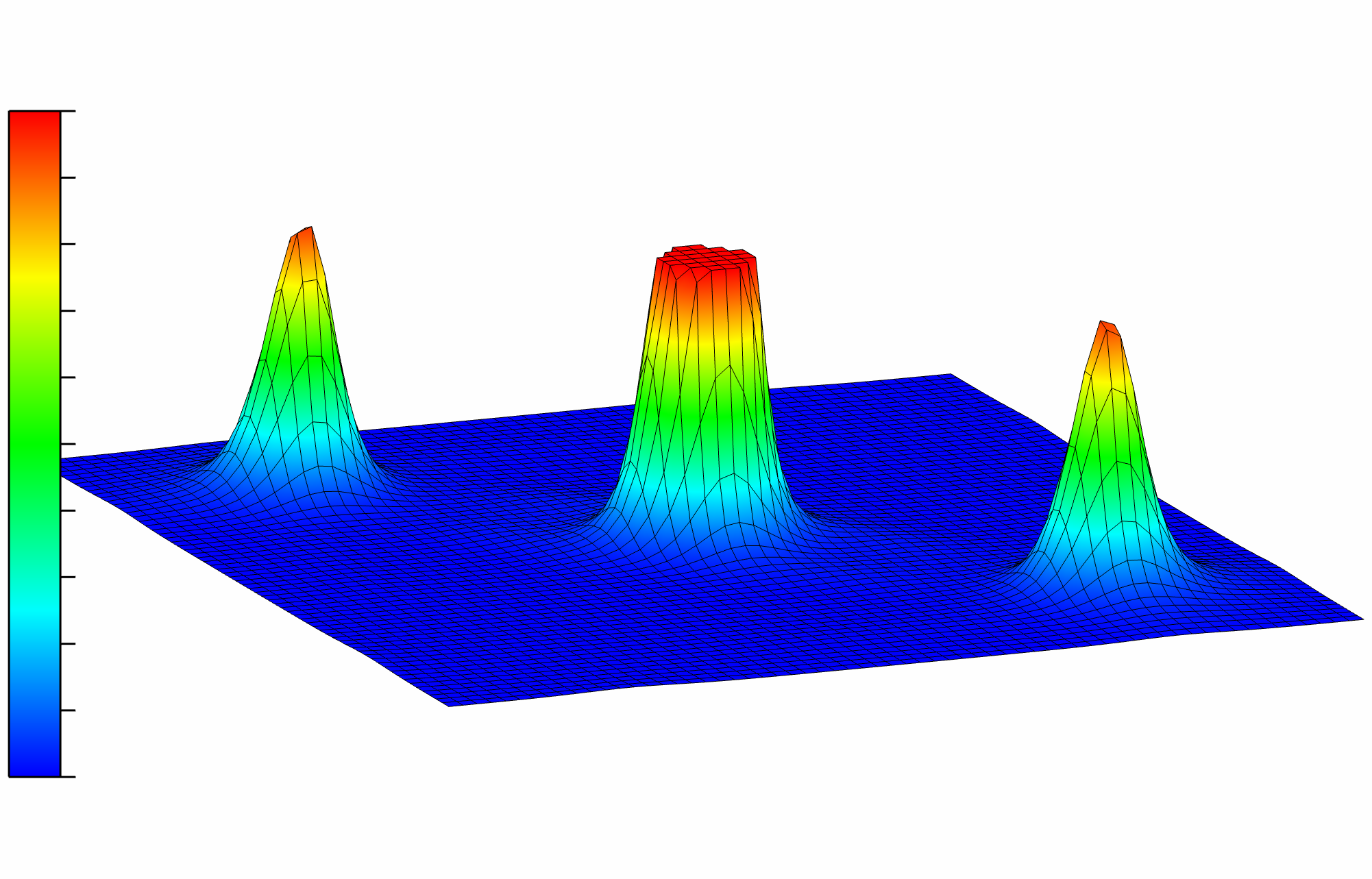
Figure 15.1 shows the 2D Data Display window of VESTA running on Windows 7.
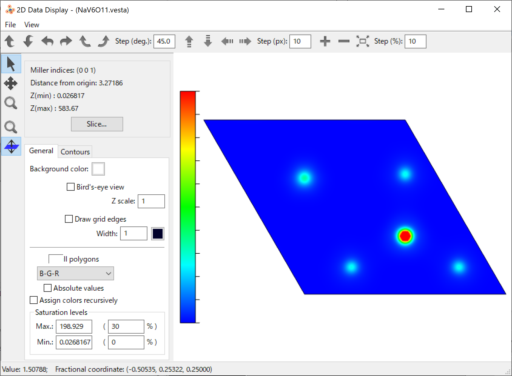
This window comprises the following four components:
- Menu bar: On Windows and Linux, the menu bar is placed at the top of the Main Window. On macOS, menus are displayed at the top of the screen. “File” and “View” menus are available in this window.
- Toolbar: Tools used frequently.
- Side Panel: Colors, contours, and other properties of a 2D image are controlled in the Side Panel. The minimum and maximum values in the 2D slice/projection data are displayed at the top of the panel.
- Graphics Area: Display an 2D image of volumetric data.
If a 2D image has been previously displayed, it is restored as soon as this window is opened. The default preferences of colors and width of contour lines, and the background color can be changed when no 2D image is displayed in this window. To change these default settings, edit values in the Side Panel and then close the window to save the settings.
15.2 Menus
- File menu
- Export 2D Data...: Export 2D data as a text file.
- Export Raster Image...: Export a graphic image as a file with a raster (pixel-based) format.
- Close: Close the 2D Data Display window.
- View menu
- Zoom In: Zoom in an image.
- Zoom Out: Zoom out an image.
15.3 Tools in the Toolbar
15.3.1 Rotation
| Rotate around the x axis | ||
| Rotate around the x axis | ||
| Rotate around the y axis | ||
| Rotate around the y axis | ||
| Rotate around the z axis | ||
| Rotate around the z axis | ||
These six buttons are used to rotate objects around one of the \(x\), \(y\), and \(z\) axes. The step width of rotation (in degrees) is specified in a text box next to the sixth button:
![]()
15.3.2 Translation
| Translate upward | ||
| Translate downward | ||
| Translate leftward | ||
| Translate rightward | ||
These four buttons are used to translate objects toward up, down, left, and right, respectively. The step width of translation (in pixels) is specified in a text box next to the fourth button:
![]()
15.3.3 Scaling
| Zoom in | ||
| Zoom out | ||
| Fit to the screen | ||
These three buttons is used to change object sizes. The step width of zooming (in %) is specified in a text box next to the third button:
![]()
15.4 Tools in the Vertical Toolbar
| Rotate | ||
| Translate | ||
| Magnify | ||
| Magnify by mouse wheel | ||
| Shift slice by mouse wheel | ||
15.5 Create and Edit a 2D Image
Click the [Slice...] button in the Side Panel to create a new image. Then, a dialog box named Create New Slice is opened (Fig. 15.2).
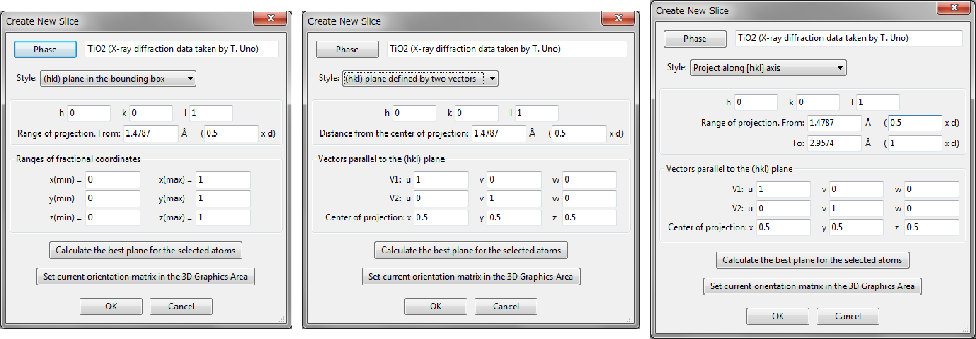
Three different methods of creating a slice or a projection image can be used:
- 1.
- (hkl) plane in the bounding box
- 2.
- (hkl) plane defined by two vectors
- 3.
- Project along [hkl] axis.
Figure 15.3 schematically illustrates how a 2D image is created in each mode.
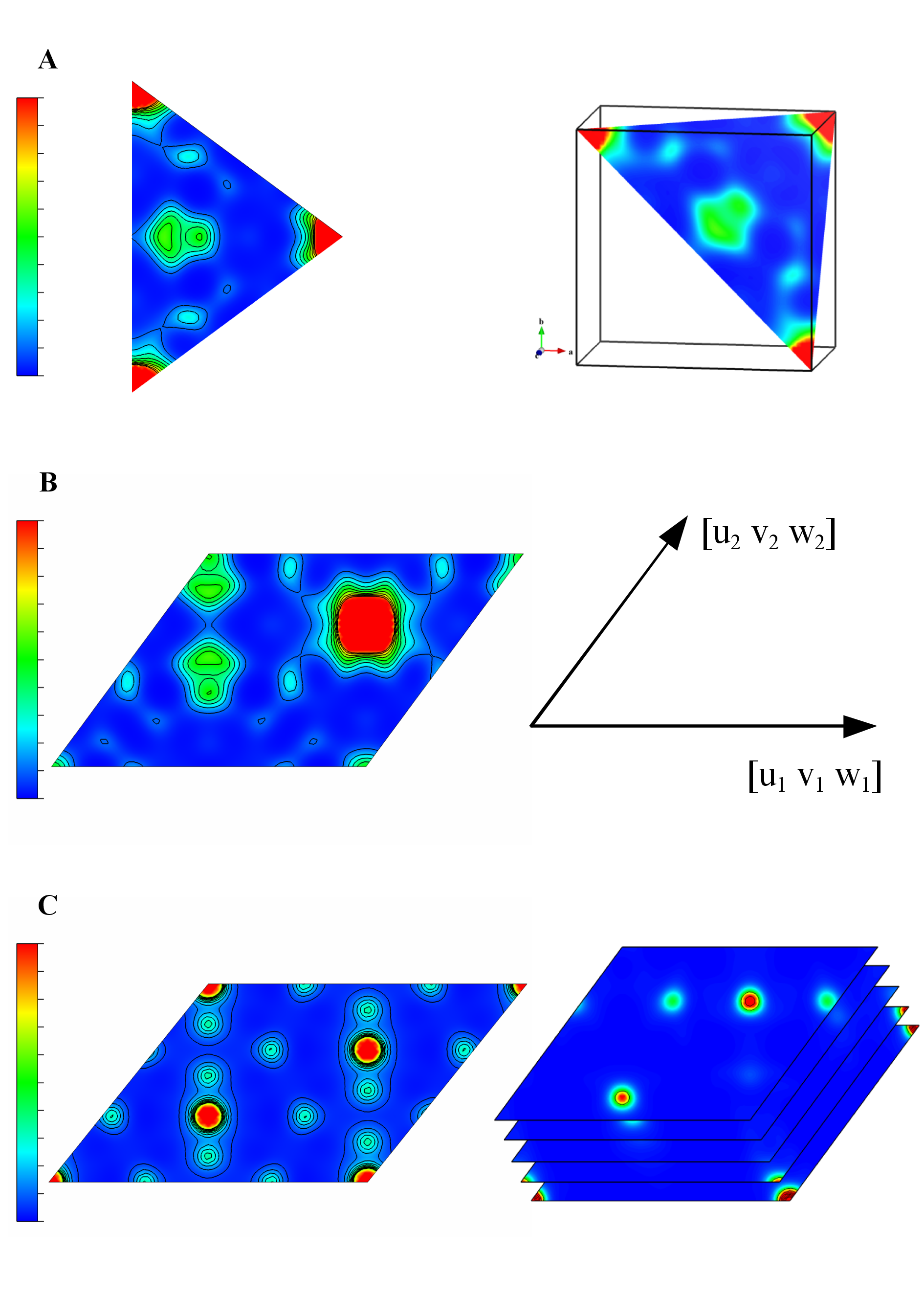
15.5.1 (hkl) plane in the bounding box
In this mode, a slice that cuts a bounding box is created. The size of the bounding box is specified by ranges along \(x\), \(y\), and \(z\) axes. The position of the slice is given as a distance from the origin of 3D data in the unit of either its lattice-plane spacing, \(d\), or Å.
15.5.2 (hkl) plane defined by two vectors
In this mode, the size of the slice is defined by two lattice vectors: \([u_1 v_1 w_1]\) and \([u_2 v_2 w_2]\).
- h, k, and l:
- Three values in an equation to represent the lattice vector, \(\bm {R} = h \bm {a} + k \bm {b} + l \bm {c}\), where \(\bm {a}\), \(\bm {b}\), and \(\bm {c}\) denote fundamental lattice vectors.
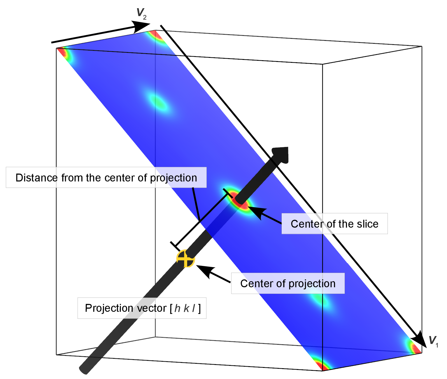
- Distance from the center of procection:
- The Center of projection lies on the projection vector that passes through the center of the slice (Fig. 15.4). The distance between the center of slice and the Center of projection is specified in the unit of either its lattice-plane spacing, \(d\), or Å. For example, when this value is 0, the (\(x\), \(y\), \(z\)) position specified as the Center of projection corresponds to the center of the slice.
- Vectors parallel to the (hkl) plane:
- A pair of vectors, \(\bm {V}_1\) and \(\bm {V}_2\), is specified in the expression of the lattice vector, \(u \bm {a} + v \bm {b} + w \bm {c}\), on the (\(hkl\)) plane. The two lattice vectors should be parallel to the (\(hkl\)) plane but should not be parallel to each other.
- Center of projection:
- Projection of this point along the [\(hkl\)] direction intersects the slice at the center of the slice.
In this mode, two-dimensional data on the slice are recalculated by linear interpolation. When the numbers of data points along \(x\), \(y\), and \(z\) directions in the volumetric data are \(N\)[0], \(N\)[1], and \(N\)[2], respectively, the number of data points, \(N_x\), along the \([u_1 v_1 w_1]\) direction is computed by \begin {equation} N_x = \mathrm {(int)}(N[0]*u_1 + N[1]*v_1 + N[2]*w_1). \end {equation} The same procedure is applied to the number of data points along the \([u_2 v_2 w_2]\) direction.
15.5.3 Project along [hkl] axis
This mode draws cumulative data of a series of (\(hkl\)) slices summed up along the [\(hkl\)] direction in a user-specified range. The number of data points is calculated in the same way as with the “(hkl) plane defined by two vectors” mode.
In the Slice Properties dialog box for this mode, four kinds of data have to be input:
- h, k, and l:
- Three values in an equation to represent the lattice vector, \(\bm {R} = h \bm {a} + k \bm {b} + l \bm {c}\), where \(\bm {a}\), \(\bm {b}\), and \(\bm {c}\) denote fundamental lattice vectors. The [\(hkl\)] direction is defined with \(\bm {R}\).
- Range of projection:
- A pair of values specified by distances from the Center of projection. They are input in the unit of either its lattice-plane spacing, \(d\), or Å.
- Vectors parallel to the (hkl) plane:
- A pair of vectors, \(\bm {V}_1\) and \(\bm {V}_2\), is specified in the expression of the lattice vector, \(u \bm {a} + v \bm {b} + w \bm {c}\), on the (\(hkl\)) plane. The two lattice vectors should be parallel to the (\(hkl\)) plane but should not be parallel to each other.
- Center of projection:
- Projection of this point along the [\(hkl\)] direction intersects the slice at the center of the slice.
15.6 Controlling Properties of a 2D Image
In the General page in the Side Panel, colors of the background and plane are mainly controlled (see Fig. 15.1).
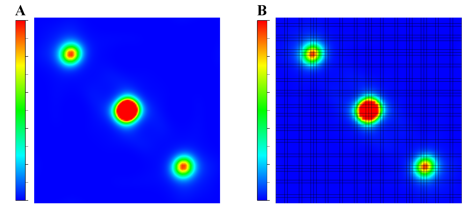
Press a button at the right side of Background color: to change the background color. Check box “Bird’s eye view” enables or disables Bird’s eye view (Fig. 15.5). If “Draw grid edges” is checked, edges of grids are drawn with solid lines of a color and a width specified below the check box (Fig. 15.6).
When “Fill polygons” is checked, the surface of the plane is filled with colors corresponding to data values. Colors of the plane are controlled in the same manner as with sections of isosurfaces (see 12.1.6).
In the Contours page (Fig. 15.7), various properties of contour lines are specified. Check “Draw contour lines” to draw contour lines, which are plotted in two different modes: linear or logarithmic.
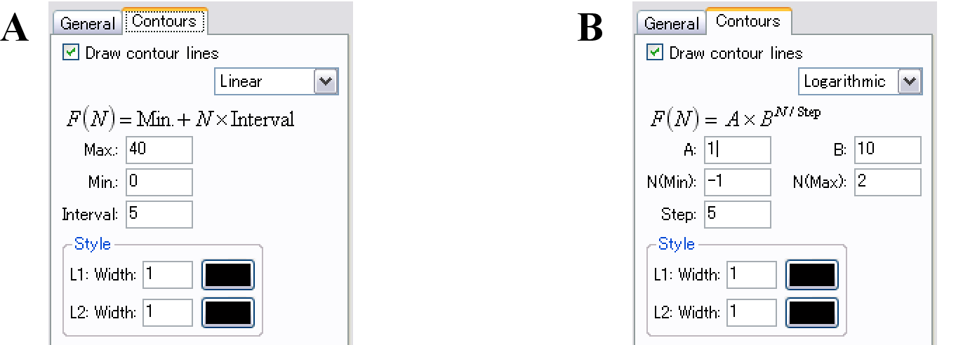
Contours are plotted in linear and logarithmic modes as solid lines (style L1) and dashed ones (style L2). The width and colors of these lines are specified in the text boxes and buttons in the Style frame box.
In the linear mode, lines are drawn at every \(\mathrm {Interval}\) in data ranging from Min. to Max. The numerical value at the \(N\)th line, \(F(N)\), is given by \begin {equation} F(N) = \mathrm {Min.} + N \times \mathrm {Interval}. \end {equation} In this mode, line style L1 (solid line) is applied to lines of positive values, and line style L2 (dashed line) to lines of negative values.
In the logarithmic mode, \(F(N)\) is computed by \begin {equation} F(N) = A \times B^{N/\mathrm {Step}}, \end {equation} where \(A\) and \(B\) are constants specified by user. Line style L1 is applied to every “step” lines starting from the first one, and for other lines the L2 style is applied. For example, when \(N_{\mathrm {min}}\) is set to an integer value, the L1 style is used for lines with integer values of \(N/\mathrm {Step}\), and the L2 style is used for lines with non-integer values of \(N/\mathrm {Step}\).
15.7 Exporting 2D data
To export 2D data of the specified slice as a text file, choose “File” menu \(\Rightarrow \) “Export 2D Data…” in the 2D Data Display window. No 2D data files can be output on selection of style “(hkl) plane in the bounding box” in the Slice Properties dialog box.
