
Chapter 10
DEFINING DRAWING BOUNDARIES AND VIEW DIRECTIONS
10.1 Drawing Boundaries
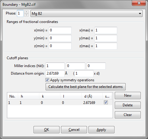
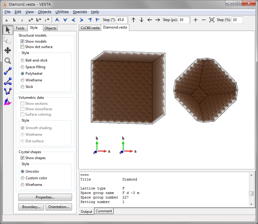
To change the size of a drawing boundary (box), select the [Boundary] button in the Side Panel, or choose “Objects” menu \(\Rightarrow \) “Boundary…”. Then, the Boundary dialog box appears as Fig. 10.1 illustrates. This dialog box can also be opened with a keyboard shortcut of \(<\)Ctrl\(>\) + \(<\)Shift\(>\) + \(<\)B\(>\). At the top of the dialog box, select a phase to edit. Press the [OK] or [Apply] button to reflect editing results in the Graphics Area.
Changing the boundary regenerates all the atoms in the Graphics Area and reset all the properties of objects to default values. Selected or hidden states of atoms, bonds, and polyhedra are reset to the default states.
10.1.1 Ranges of fractional coordinates
Drawing boundaries are fundamentally specified by inputting ranges of fractional coordinates along \(x\), \(y\), and \(z\) axes.
10.1.2 Cutoff planes
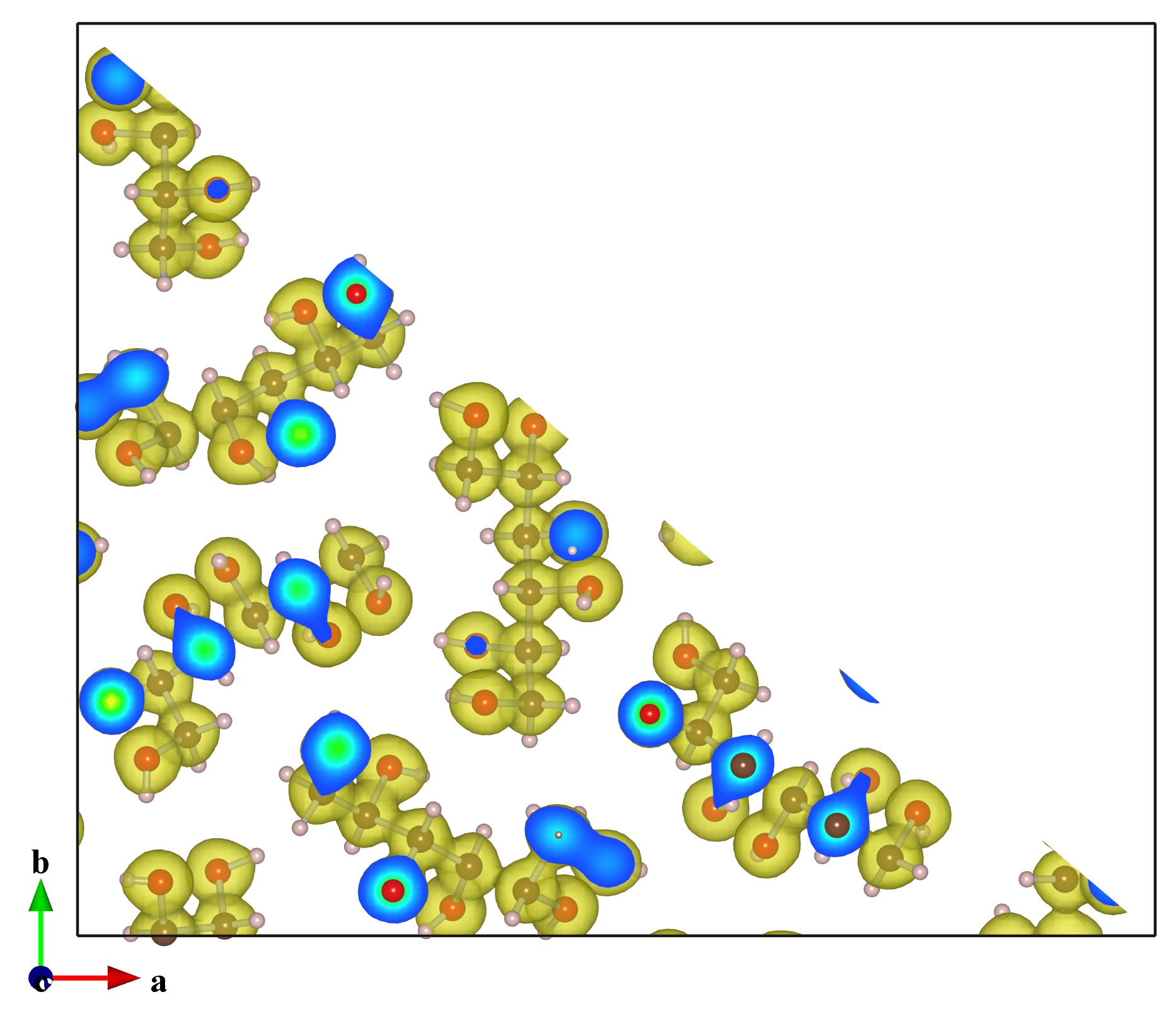
In addition to ranges of fractional coordinates, we can further specify “cutoff planes,” as exemplified in Fig. 10.2. After atoms, bonds, and isosurfaces within the \(x\), \(y\), and \(z\) ranges have been generated, those lying outside of the cutoff planes are excluded. Even though atoms, bonds, and polyhedra can be hidden by another procedure described in 11.4, this is the only way to remove part of isosurfaces and sections. This feature is, therefore, particularly useful for visualizing 2D distribution of volumetric data on lattice planes in addition to isosurfaces. Each cutoff plane is specified as Miller indices \(hkl\) and a distance from the origin, (0, 0, 0). The distance of a cutoff plane from the origin may be specified in the unit of either its lattice-plane spacing, \(d\), or Å.
When option “Apply symmetry operations” is checked, all the symmetrically equivalent Miller planes are used as cutoff planes (Fig. 10.3). To define a cutoff plane with selected atoms, select three or more atoms in the Graphics Area and press the [Calculate the best plane for the selected atoms] button.
The Cutoff planes frame box lists cutoff planes. Some of buttons and text boxes are disabled when no cutoff plane is selected in the list. On selection of an item in the list, the text boxes are updated to show data relevant to the selected cutoff plane. To add a new cutoff plane, click the [New] button at first, and input Miller indices, \(hkl\), and the distance from the origin. To delete a cutoff plane, select an item in the list, and then click the [Delete] button or press the \(<\)Delete\(>\) key. Clicking the [Clear] button deletes all the cutoff planes in the list.
10.2 View Direction
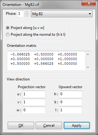
To specify a direction of viewing objects, select the [Orientation] button in Side Panel, or choose “Objects” menu \(\Rightarrow \) “Orientation…”. Then, the Orientation dialog box appears as Fig. 10.4 shows. This dialog box can also be opened with a keyboard shortcut of \(<\)Ctrl\(>\) + \(<\)Shift\(>\) + \(<\)O\(>\). At the top of the dialog box, specify a phase to which the viewing direction is applied. To change relative orientation of each phase, use the Phase tab in the Edit Data dialog box (see chapter 7).
10.2.1 Manner of specifying directions
Either a lattice vector, \([uvw]\), or a reciprocal-lattice vector, \([hkl]^*\), perpendicular to a lattice plane \((hkl)\) is specified as the direction of projection.
- Project along [uvw]
The direction of projection is a lattice vector \(ua + vb + wc\). - Project along the normal to (hkl)
The direction of projection is a reciprocal-lattice vector \(ha^* + kb^* + lc^*\).
10.2.2 Orientation matrix
A \(3 \times 3\) rotation matrix of the current orientation is displayed.
10.2.3 View direction
Two directions, i.e., the direction of projection (direction from the viewpoint to the screen) and the upward direction on the screen are specified by a set of a lattice vector and a reciprocal-lattice vector. The two vectors are perpendicular to each other. When the lattice vector, \(ua + vb + wc\), lies on the \((hkl)\) plane, \(u\), \(v\), \(w\), \(h\), \(k\), and \(l\) must satisfy the condition: \begin {equation} \label {head:eqn_hukvlw_0} hu + kv + lw = 0 . \end {equation} This condition must, therefore, be satisfied in order to specify the upward direction on the screen, otherwise the upward direction on the screen is automatically determined by VESTA.
- Projection vector: Direction of projection.
In the “Project along [uvw]” mode, this vector is \(u\), \(v\), and \(w\) in \(ua + vb + wc\).
In the “Project along the normal to (hkl) plane” mode, this vector is \(h\), \(k\), and \(l\) in \(ha^* + kb^* + lc^*\). - Upward vector: Upward direction on the screen.
In the “Project along [uvw]” mode, this vector is \(h\), \(k\), and \(l\) in \(ha^* + kb^* + lc^*\).
In the “Project along the normal to (hkl) plane” mode, this vector is \(u\), \(v\), and \(w\) in \(ua + vb + wc\).
10.2.4 Viewing along crystallographic axes
![]()
![]()
![]()
![]()
![]()
![]()
To view the contents of Graphics Area along basis vectors of a unit cell or a reciprocal cell, simply press one of the above buttons in the Horizontal Toolbar. When two or more phases are visualized in the same Graphics Area, the above buttons set the viewing direction relative to the first phase. To set a viewing direction relative to a phase other than the first one, use the Orientation dialog box.
